Tree Cover Loss Analysis

Tree Cover Loss Analysis#

Step 1. Import Libraries#

import pandas as pd
import seaborn as sns
import matplotlib.pyplot as plt
from IPython.display import display, Markdown, Latex, Image

Step 2. Prepare data from Global Forest Watch #

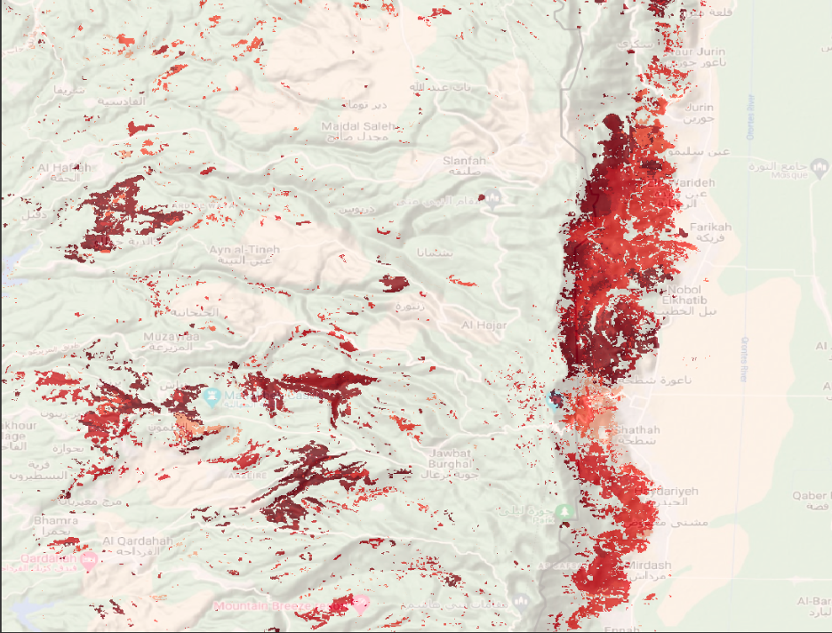
Global forest watch sources its data from a University of Maryland time-series analysis of Landsat images that show global forest extent and change. These data can be downloaded for free, as .tiff files.

Following is an example of what these files look like rendered using QGIS, in Syria, covering the period from 2000-2020. The intensity of the red color is commensurate with the intensity of forest cover loss.

Image("images/syria-tree-loss-2.png")

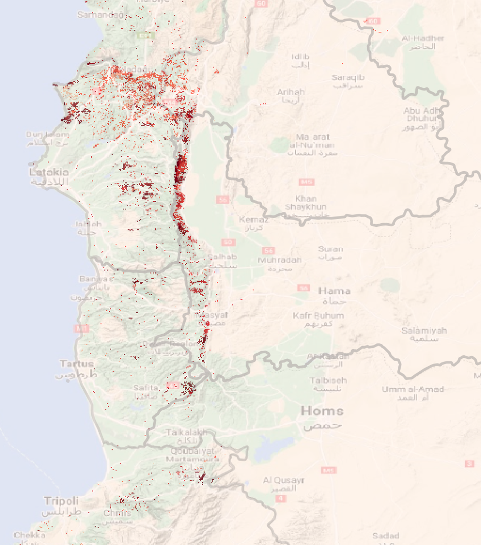
../../_images/6f811f3d313f4e207103d30875dedcba0434b2eb7c3aced4d262c64da9e659d0.png

Image("images/syria-tree-loss-3.png")

../../_images/3678a2e600f13b4a3d739f51f20832f6f6d7a566429e6b4acc0ccef3b237943d.png

# Read in treecover data loss dataset and metadata. The metadata will help us match admin id numbers with their actual names
df = pd.read_csv("data/treecover_loss_by_region__ha.csv")
meta = pd.read_csv("data/adm1_metadata.csv", usecols=["name", "adm1__id"])

# Merge data frames on adm1 column
merged_df = pd.merge(df, meta, left_on="adm1", right_on="adm1__id", how="left")

# Drop original adm1 column and rename merged adm1 column to "adm1"
merged_df.drop("adm1", axis=1, inplace=True)
merged_df.rename(columns={"name": "adm1"}, inplace=True)

# Preview the new merged data frame
merged_df.head()

	iso	umd_tree_cover_loss__year	umd_tree_cover_loss__ha	gfw_gross_emissions_co2e_all_gases__Mg	adm1	adm1__id
0	SYR	2001	3.480518	763.156831	Al Ḥasakah	1
1	SYR	2001	23.259127	5419.176101	Aleppo	2
2	SYR	2001	7.879289	1948.088177	Ar Raqqah	3
3	SYR	2001	2.140265	545.701701	Dayr Az Zawr	7
4	SYR	2001	75.270909	20104.074759	Hamah	8

Step 3. Create pivot table to show change in forest cover loss over time, by first administrative level#

# Create pivot table of tree cover loss by admin1 and year
pivot = pd.pivot_table(merged_df, values="umd_tree_cover_loss__ha",
                       index="adm1", columns="umd_tree_cover_loss__year",
                       aggfunc=sum, fill_value=0)

# Display the pivot table
display(pivot)

umd_tree_cover_loss__year	2001	2002	2003	2004	2005	2006	2007	2008	2009	2010	...	2012	2013	2014	2015	2016	2017	2018	2019	2020	2021
adm1
Al Ḥasakah	3.480518	0.986151	0.862637	0.123263	0.061612	0.062083	0.000000	2.227976	0.309338	0.868839	...	1.489113	0.370907	0.124082	0.000000	0.000000	0.000000	0.000000	0.000000	0.000000	0.000000
Aleppo	23.259127	2.558609	14.358696	7.035085	6.465869	4.662156	7.333947	120.965704	18.725133	4.921604	...	16.887510	37.336229	19.853886	0.994854	1.116550	7.650396	25.461913	123.576922	109.802907	82.457021
Ar Raqqah	7.879289	4.689905	1.565029	1.188662	0.874299	1.432591	2.629462	2.128434	4.065437	6.387455	...	2.317495	0.436470	0.125291	0.250553	0.000000	0.000000	0.000000	0.000000	0.000000	0.000000
Dar`a	0.000000	0.000000	0.000000	0.000000	0.000000	0.000000	0.000000	0.000000	0.000000	0.000000	...	0.000000	0.064731	0.258925	0.000000	0.064732	0.000000	0.000000	0.000000	0.000000	0.000000
Dayr Az Zawr	2.140265	0.188467	0.377624	0.696905	0.126386	0.000000	1.073532	0.762680	0.568986	0.251701	...	1.319054	0.314921	0.000000	0.000000	0.000000	0.000000	0.000000	0.000000	0.000000	0.000000
Hamah	75.270909	21.656590	8.800606	8.246462	9.514644	155.613112	24.385281	12.506246	30.970247	34.212082	...	207.689804	158.491165	259.917182	1634.596085	1125.643516	1105.887974	425.235510	481.166452	1202.593810	536.263460
Hims	6.352807	0.507980	0.381551	0.253918	2.792863	0.317257	1.904211	0.127070	2.094730	1.143021	...	2.923788	4.262075	4.062676	43.459727	92.174943	23.728053	4.188380	4.507124	74.919512	183.112050
Idlib	27.095845	15.280434	24.910104	14.464419	12.279044	46.664039	34.823248	10.393510	7.070212	113.332822	...	1106.759225	74.325848	109.792240	93.491690	115.755690	311.652435	186.094799	131.866447	84.258604	55.678079
Lattakia	76.985513	88.706425	54.998993	71.267972	742.447252	65.291268	1480.024060	668.021859	54.883082	69.666617	...	4022.257680	968.074040	522.129303	501.735361	426.535367	588.007699	235.497610	351.082340	1356.140526	1622.487838
Rif Dimashq	1.610330	0.193247	0.193407	0.579396	1.417245	0.000000	0.128872	0.000000	0.064410	0.064413	...	0.064207	0.000000	0.000000	0.000000	0.000000	0.000000	0.000000	0.000000	0.000000	0.000000
Tartus	43.160692	13.231385	8.357694	3.166264	15.828417	6.709051	24.934269	17.024264	12.155203	9.684413	...	8.933851	26.756466	42.030749	118.642899	51.382905	109.643047	26.950682	84.320991	209.955002	376.116621

11 rows × 21 columns

Step 4. Calculate cumulative forest cover loss#

import matplotlib.ticker as ticker
import matplotlib.pyplot as plt

# Set font family
plt.rcParams['font.family'] = 'sans-serif'

# Group data by admin1 and year, and calculate cumulative tree cover loss
grouped_df = merged_df.groupby(['adm1', 'umd_tree_cover_loss__year'])['umd_tree_cover_loss__ha'].sum().reset_index()
grouped_df['cummulative loss'] = grouped_df.groupby('adm1')['umd_tree_cover_loss__ha'].cumsum()

# Convert year column to integers
grouped_df['umd_tree_cover_loss__year'] = pd.to_numeric(grouped_df['umd_tree_cover_loss__year'], errors='coerce', downcast='integer')

# Replace NaN values with None
grouped_df['umd_tree_cover_loss__year'] = grouped_df['umd_tree_cover_loss__year'].where(pd.notnull(grouped_df['umd_tree_cover_loss__year']), None)

# Create line chart of cumulative tree cover loss over time, by admin1
plt.figure(figsize=(24,12))
ax = sns.lineplot(x='umd_tree_cover_loss__year', y='cummulative loss', hue='adm1', data=grouped_df, linewidth=3)
ax.set_xlabel('Year', fontsize=16)
ax.set_ylabel('Cumulative Tree Cover Loss (ha)', fontsize=16)
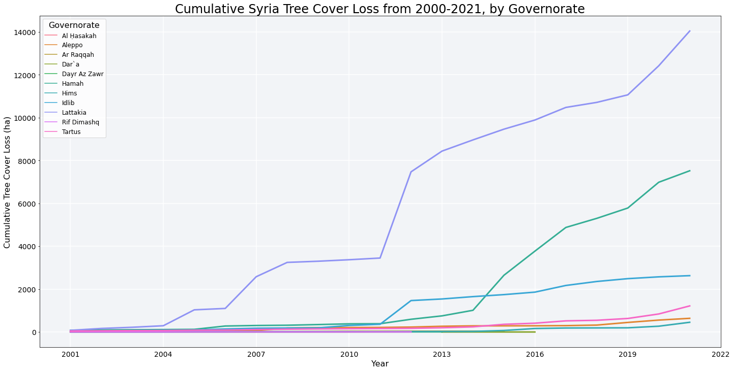
ax.set_title('Cumulative Syria Tree Cover Loss from 2000-2021, by Governorate', fontsize=24)
ax.tick_params(labelsize=14)
ax.legend(fontsize=12, title='Governorate', title_fontsize=16)
ax.xaxis.set_major_locator(ticker.MaxNLocator(integer=True))

# Set background color and grid
ax.grid(True, 'major', axis='y', color='w', linestyle='-', linewidth=1.5)
ax.set_facecolor('#F2F4F7')
ax.xaxis.grid(True, which='major', color='w', linestyle='-', linewidth=1.5)
ax.xaxis.set_tick_params(width=0)

# Save chart as a PNG file
plt.savefig('images/syria-tree-loss-chart.png', dpi=300, bbox_inches='tight')

plt.show()

../../_images/4454f50a5cddb57e3ca63d44d319736bb6ac8afa635394f487930ae7591c4d5d.png

Step 5. Calculate total tree cover loss by administrative level 1, identify which admin1s account for the greatest losses, and then calculate their percent of the national total#

# Group data by admin1 and calculate tree cover loss
total_loss = round (merged_df.groupby('adm1')['umd_tree_cover_loss__ha'].sum(),2)

# Calculate percentage of the total tree cover loss for each admin1
percentage_loss = total_loss / total_loss.sum() * 100

# Get the admin1 with the highest tree cover loss
most_loss = total_loss.idxmax()
percentage_of_total = percentage_loss.max()

# Get the admin1 with the second highest tree cover loss
second_most_loss = total_loss.nlargest(2).iloc[-1]
second_most_loss_adm1 = total_loss.nlargest(2).index[-1]
percentage_of_total_2 = percentage_loss[second_most_loss_adm1]

# Get the admin1 with the third highest tree cover loss (repeat for additional areas)
third_most_loss = total_loss.nlargest(3).iloc[-1]
third_most_loss_adm1 = total_loss.nlargest(3).index[-1]
percentage_of_total_3 = percentage_loss[third_most_loss_adm1]

# Display the results (customize the local name for an admin1 area)

display(Markdown(f"The governorate with the most tree cover loss is {most_loss}, with {total_loss[most_loss]} hectares lost, which represents {percentage_of_total:.2f}% of the total loss across all governorates."))
display(Markdown(f"The governorate with the second most tree cover loss is {second_most_loss_adm1}, with {second_most_loss} hectares lost, which represents {percentage_of_total_2:.2f}% of the total loss across all governorates."))
display(Markdown(f"The governorate with the third most tree cover loss is {third_most_loss_adm1}, with {third_most_loss} hectares lost, which represents {percentage_of_total_3:.2f}% of the total loss across all governorates."))

The governorate with the most tree cover loss is Lattakia, with 14045.48 hectares lost, which represents 52.85% of the total loss across all governorates.

The governorate with the second most tree cover loss is Hamah, with 7524.2 hectares lost, which represents 28.31% of the total loss across all governorates.

The governorate with the third most tree cover loss is Idlib, with 2629.7 hectares lost, which represents 9.90% of the total loss across all governorates.

NOTE: Most of the code in this workbook was generated using a ChatGPT notebook prepred by the Lab: https://holly-transport.github.io/coffee_chat/notebooks/CoffeeChat.html