Calculate Number of Devices within Areas of Interest

In this step, we calculate the number of devices detected within the areas of interest, creating a time series.

Show code cell content Hide code cell content

import dask.dataframe as dd
import geopandas
import matplotlib.dates as mdates
import matplotlib.pyplot as plt
import pandas as pd
import humanize
from dask.distributed import Client

# https://papermill.readthedocs.io/en/latest/usage-parameterize.html
DASK_SCHEDULER_ADDRESS = None

AOI = "id=7&name=A"
NAME = "A"

Data

Area of Interest

AOI = geopandas.read_file(f"../../data/interim/aoi/{AOI}.geojson")

Mobility Data

In this step, we import the panel of devices detected within the area of interest.

PATH = [
    f"../../data/interim/panels/{NAME}",
]

filters = []

Reading the mobility data as an Apache Parquet Dataset in parallel using Dask,

ddf = dd.read_parquet(PATH, filters=filters)

Filtering,

ddf = ddf[ddf["h3_10"].isin(AOI["hex_id"])]

Exploratory Data Analysis

First, let’s just take a look!

# dropping uid, for privacy
ddf.head().drop(["uid"], axis="columns")

	latitude	longitude	h3_10	datetime	date	country	year	quarter
6934	34.637413	35.975620	8a2da225baeffff	2020-01-01 17:39:01+02:00	2020-01-01	LB	2020	1
24842	34.637543	35.976097	8a2da35a6db7fff	2020-01-02 17:54:28+02:00	2020-01-02	LB	2020	1
29011	34.664909	36.308998	8a2da348d807fff	2020-01-02 18:16:56+02:00	2020-01-02	LB	2020	1
29021	34.664909	36.308998	8a2da348d807fff	2020-01-02 18:01:56+02:00	2020-01-02	LB	2020	1
29022	34.664909	36.308998	8a2da348d807fff	2020-01-02 17:40:52+02:00	2020-01-02	LB	2020	1

humanize.naturalsize(ddf.memory_usage(deep=True).sum().compute())

'89.6 MB'

As seen, the data will easily fit in memory. Let’s convert to a pandas.DataFrame.

df = ddf.compute()

len(df)

306785

And now, a sneak peek of 10,000 locations from the panel.

gdf = geopandas.GeoDataFrame(
    df[["longitude", "latitude"]].iloc[:10000],
    geometry=geopandas.points_from_xy(
        df.longitude.iloc[:10000], df.latitude.iloc[:10000], crs="EPSG:4326"
    ),
)
gdf.explore()

Make this Notebook Trusted to load map: File -> Trust Notebook

Important

This is a partial disclosure. Additional content in this section was suppressed from this notebook to adhere to the data classification policy.

Generate Time Series

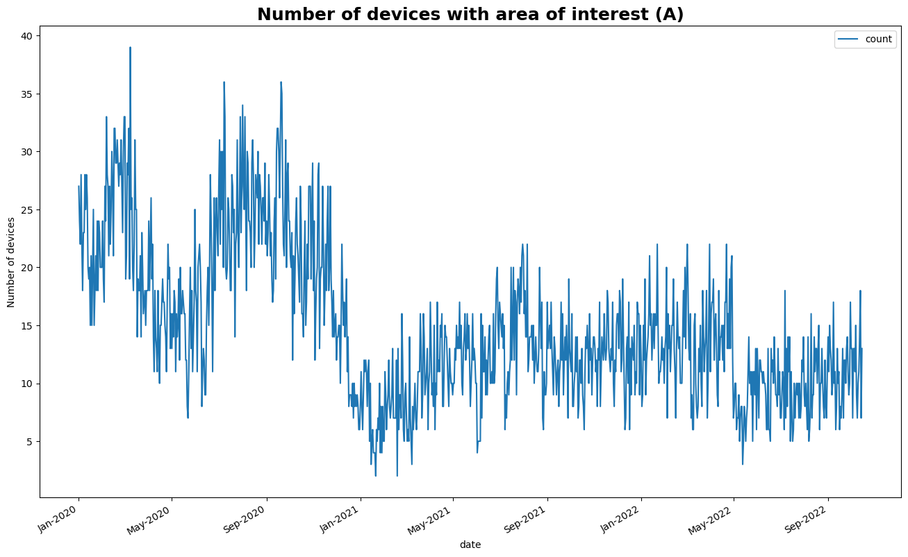
Now, we are interested to see how the number of devices evolves in time. Let’s calculate the daily number of devices detected withih the area of interest.

count = ddf.groupby(["date"])["uid"].nunique().compute().to_frame("count")

count.index = pd.to_datetime(count.index)

Plotting,

Show code cell source Hide code cell source

fig, ax = plt.subplots(figsize=(16, 10))

count.plot(ax=ax)
ax.set_title(
    f"Number of devices with area of interest ({NAME})",
    fontsize=18,
    fontweight="bold",
)
ax.yaxis.set_label_text("Number of devices")
ax.xaxis.set_major_formatter(mdates.DateFormatter("%b-%Y"));