Analysing Spatial Distribution of Conflict before and after the fall of the Assad Regime

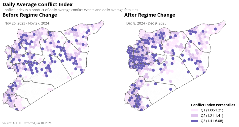
Mean Conflict Index

The conflict intensity index is calculated as the geometric mean of conflict events and fatalities, with an adjustment to handle zero values:

\[\text{Conflict Intensity Index} = \sqrt{(\text{nrEvents}) \times (\text{nrFatalities} + 1)}\]

Where:

• \(\text{nrEvents}\) is the number of conflict events in a given period and location

• \(\text{nrFatalities}\) is the number of fatalities from conflicts in the same period and location

• The addition of 1 to each term ensures the index is defined even when either component is zero. This is arbitrary and is doen just to account for 0 values of fatalities and conflicts.

This index provides a balanced measure that accounts for both the frequency of conflicts and their severity. Compared to arithmetic means, the geometric mean reduces the influence of extreme values in either component (conflict events + fatalities). Areas with both high events and high fatalities will have higher index values than areas with many events but few fatalities or vice versa.

Conflict index is calculated at the location and then average is taken over time (across the three time periods). This is to preserve the integrity of the conflict index in that specific location.

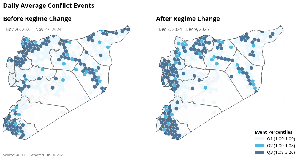
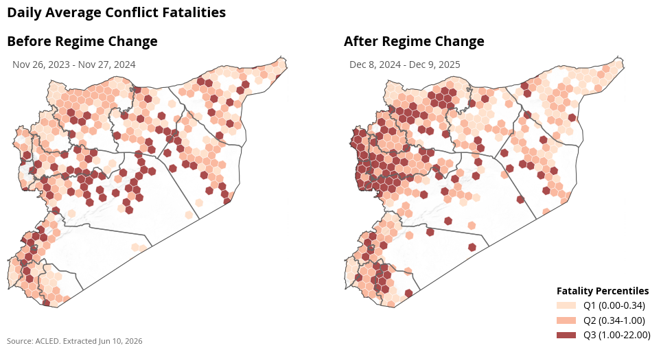
Spatial Distribution of Average Daily Conflict

/Users/ssarva/syria-economic-monitor/.venv/lib/python3.13/site-packages/IPython/core/events.py:82: UserWarning: Glyph 8594 (\N{RIGHTWARDS ARROW}) missing from font(s) Open Sans.
  func(*args, **kwargs)

/Users/ssarva/syria-economic-monitor/.venv/lib/python3.13/site-packages/IPython/core/pylabtools.py:170: UserWarning: Glyph 8594 (\N{RIGHTWARDS ARROW}) missing from font(s) Open Sans.
  fig.canvas.print_figure(bytes_io, **kw)

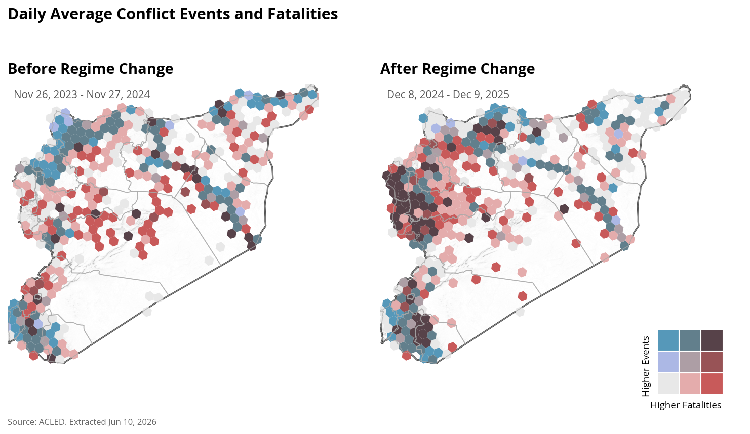
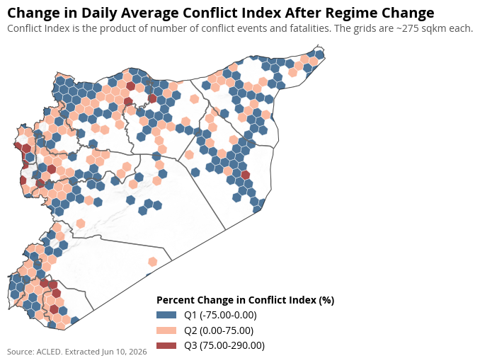
The average conflict events and conflict fatalities per day has increased in the Lattakia, of the country after regime change. In some parts around Damascus the conflicts reduced, while they increased in others.

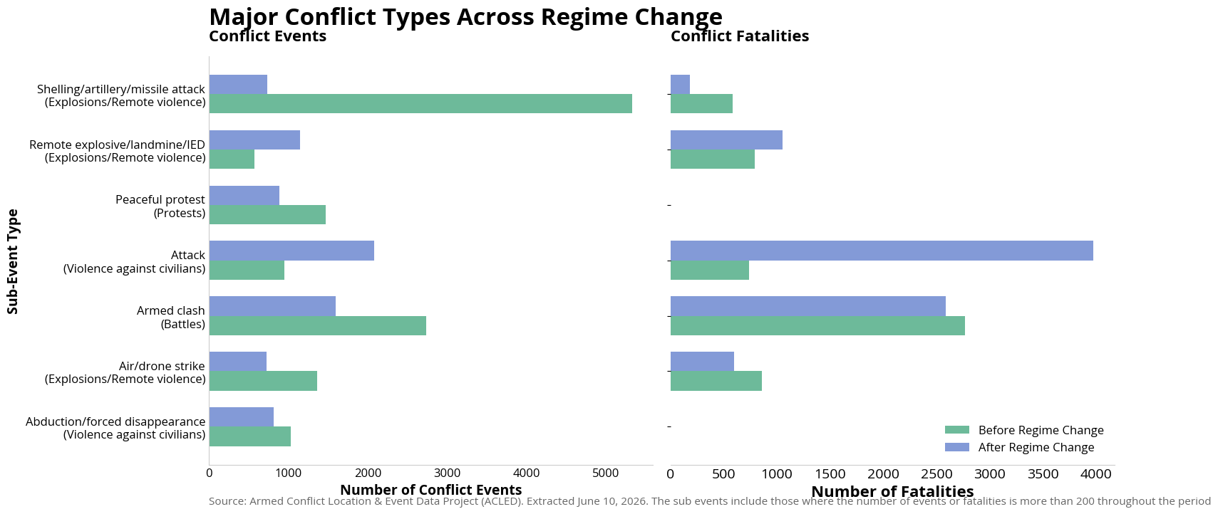
Major Conflict Types

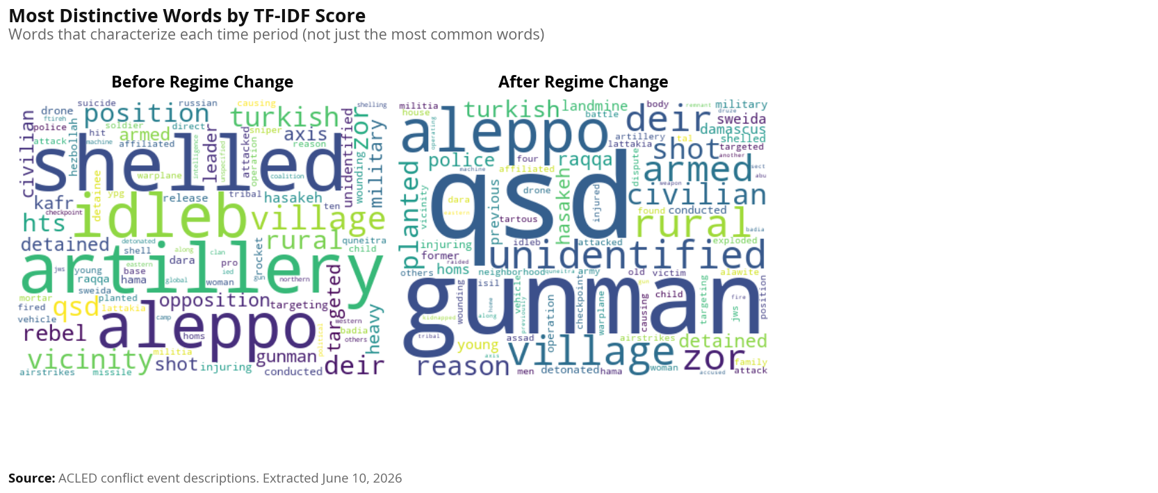
Major Conflict Topics

This section uses natural language processing to identify distinct protest topics/themes:

Method: TF-IDF (Term Frequency-Inverse Document Frequency) with K-means clustering identifies groups of conflict events that share similar language and themes.

Process:

1. Text Preprocessing: Apply word normalization and custom stopwords to clean the data

2. TF-IDF Vectorization: Convert text to numerical features, weighting words by their importance

Time Period Analysis: We run this analysis separately for before and after regime change

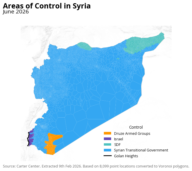
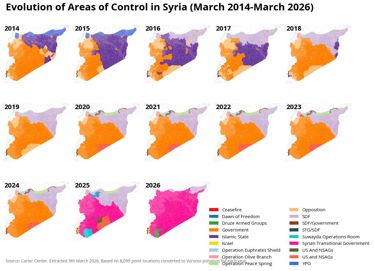
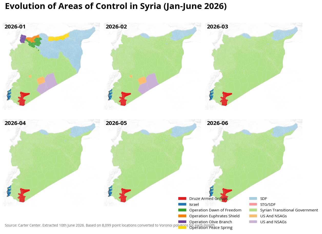
Syrian Areas of Control