Enhanced Vegetation Index and GDP Agriculture#
Literature Review: Remote Sensing for Agricultural Yield Prediction#
Enhanced Vegetation Index is the greenness or health of a pixel calculated by the MODIS Terra and Aqua satellites. This is typically used as a proxy for the health of a plant.
The relationship between crop yields and the Enhanced Vegetation Index (EVI), a proxy for vegetation health derived from satellite imagery, is central to agricultural forecasting [Johnson, 2016]. EVI is a spectral index that utilizes the blue, red, and near-infrared (NIR) bands of satellite data to monitor vegetation health. Relative to other vegetation indices, such as the Normalized Difference Vegetation Index (NDVI), EVI provided superior performance by offering increased sensitivity in high biomass areas and mitigating atmospheric effects [Huete et al., 2002]. Johnson [2016] provides a comprehensive overview of the use of EVI in agricultural yield prediction, highlighting its advantages over other indices like the Normalized Difference Vegetation Index (NDVI). The study concluded that EVI was among the best overall performer in predicting crop yields, showing the highest correlation in five out of nine crops studied, excluding rice.
Numerous studies have successfully utilized EVI to predict yields of various crops, including maize, soybeans, and rice. For instance, Bolton and Friedl [2013] created a linear model using EVI to forecast soybean and maize yields in the Central United States. Their findings demonstrate that EVI exhibits a stronger correlation with maize yield and yield anomalies than other vegetation indices, and incorporating phenological data significantly enhances the model’s performance. A study in Thailand by Wijesingha et al. [2015] investigated the use of MODIS EVI for rice crop monitoring and yield assessment. Their research revealed that maximum EVI achieved a high correlation of 0.95 with rice yield, indicating its effectiveness in yield prediction. Furthermore, Son et al. [2013] used MODIS EVI data for rice yield prediction in the Vietnamese Mekong Delta, reporting high correlation coefficients (R2 of 0.70 for spring-winter and 0.74 for autumn-summer in 2013, and 0.62-0.71 and 0.4-0.56 in 2014, respectively). Lastly, a study in one of the major rice-producing areas in China, Yangtze River Delta region, by Shi and Huang [2015] further confirmed that the MODIS-based area shows higher consistency with agricultural census data during the period of 2000-2010, with less than 15% error.
Both NDVI and EVI have been used to study agricultural productivity and EVI.
We consider the assumption that EVI can be a proxy for crop yield and thereby hypoythesize that it will have a relationship to agricultural GDP. The subsequent insights analyse the relationship between EVI and Agricultural GDP in Myanmar.
Satellite and Ground-Based Approaches#
Compared to ground-based methods, such as field interviews and crop cuttings, Remote sensing approach has several advantages on estimating crop yields:
Timeliness and Rapid Assessment: Remote sensing offers real-time or near real-time assessment of crop conditions and potential yields, which is crucial for situations like natural disasters or conflicts [Doraiswamy et al., 2003].
Extensive Spatial Coverage and Granularity: Satellite imagery can consistently cover large geographic areas, providing granular, field, and village-level data that can be aggregated to higher administrative levels, such as districts or provinces [Azzari et al., 2017, Becker-Reshef et al., 2010].
Cost-Effectiveness: Remote sensing is generally more cost-effective for collecting agricultural data over large areas compared to ground-based methods [Johnson, 2016, Rahman et al., 2009].
Accessibility in Difficult or Dangerous Areas: Remote sensing provides a reliable option for data collection in zones that are difficult, dangerous, or inaccessible for in-situ surveys, such as conflict areas [Jaafar and Ahmad, 2015].
Independent and Consistent Data Source: Remote sensing offers an independent data source that can validate or complement ground-based data, which may be subject to biases or inaccuracies.
However, remote sensing also has several limitations:
Spatial Resolution Limitations: While modern sensors offer higher resolutions, coarse resolution data may not accurately reflect ground situations for small agricultural clusters, small parcels, or low-intensity agriculture [Kibret et al., 2020].
Significant Computational Demands: Analyzing high-resolution imagery requires massive amounts of computational power and storage, which can be expensive and time-consuming [Petersen, 2018].
Interpretability and Bias Concerns: Satellite-derived metrics may not fully capture all determinants of crop production and may not quantitatively interpret crop growth status [Wu et al., 2023].
While remote sensing offers timely, broad-scale, and cost-effective monitoring, particularly in data-scarce or inaccessible regions, it faces challenges with resolution limitations, computational demands, and potential biases in interpreting crop conditions.
EVI and Other Vegetation Indices#
Within the remote sensing approach itself, multiple vegetation indices have been utilized to enhance the accuracy of yield predictions. Compared to other vegetation indices, EVI offers several advantages over other vegetation indices:
Reduced saturation: EVI does not saturate as quickly as NDVI at higher crop leaf area or in areas with large amounts of biomass, providing improved sensitivity in dense vegetation conditions [Huete et al., 2002]. This is crucial as high saturation in indicators like NDVI can lead to unreliable yield estimates [Son et al., 2013].
Atmospheric and Soil Correction: EVI incorporates a soil adjustment factor and corrections for the red band due to aerosol scattering, making it more resistant to atmospheric influences and soil background noise compared to NDVI [Jurečka et al., 2018].
On the other hand, EVI also has some limitations compared to other vegetation indices:
Temporal Resolution and Latency: While EVI is disseminated at 250m resolution, it may only be available at 16-day time steps, compared to NDVI’s 8-day availability, which could introduce latency issues for real-time monitoring [Johnson, 2016].
Mixed Pixel Problems: Coarse spatial resolution of MODIS EVI (250m or 500m) can limit performance in regions with small, fragmented parcels [Kibret et al., 2020].
Climate influenced on EVI#
EVI values are influenced by several environmental factors. EVI is sensitive to rainfall patterns, as the variations of phenological stages of crops, such as the timing of planting and harvesting, are closely linked to rainfall [Kibret et al., 2020]. Additionally, while EVI is designed to be resistant to atmospheric aerosols, cloud contamination, particularly during wet seasons, can affect vegetation greenness signals and lower the accuracy of yield predictions [Son et al., 2013].
Modelling Approaches of EVI#
Several modeling approaches have been successfully employed with EVI data for crop yield prediction. Statistical models, particularly linear and quadratic regression, are widely used due to their fewer data requirements and assumptions compared to biophysical models [Ji et al., 2022]. Linear regression models are frequently applied, with EVI generally performing well and showing more linear relationships with yields than NDVI for certain crops [Tiruneh et al., 2023]. Machine learning approaches have also proven effective, with [Kibret et al., 2020] applied Random Forest algorithm to MODIS EVI time series for agricultural land use classification and cropping system identification. [Pham et al., 2022] demonstrated that integrating Principal Component Analysis (PCA) with machine learning methods (PCA-ML) on VCI data effectively addresses spatial variability and redundant data issues, enhancing prediction accuracy by up to 45% in rice yield forecasting for Vietnam.
Data and Assumptions#
Data#
The following datasets are utilized in this analysis for calculating and mapping crop productivity over the past years:
Dynamic World Dataset:
Source: Dynamic World - Google and the World Resources Institute (WRI)
Description: The Dynamic World dataset provides a near real-time, high-resolution (10-meter) global land cover classification. It is derived from Sentinel-2 imagery and utilizes machine learning models to classify land cover into nine distinct classes, including water, trees, grass, crops, built areas, bare ground, shrubs, flooded vegetation, and snow/ice. The dataset offers data with minimal latency, enabling near-immediate analysis and decision-making.
Spatial Resolution: 10 meters.
Temporal Coverage: Data is available since mid-2015, updated continuously as Sentinel-2 imagery becomes available capturing near Real-time.
MODIS Dataset:
Source: NASA’s Moderate Resolution Imaging Spectroradiometer MODIS on Terra and Aqua satellites.
Description: The MODIS dataset provides a wide range of data products, including land surface temperature, vegetation indices, and land cover classifications. It is widely used for monitoring and modeling land surface processes.
Spatial Resolution: 250 meters.
Temporal Coverage: Data is available from 2000 to the present, with daily to 16-day composite products.
GDP and Agricultural Data:
Source: Official government statistics and international databases.
Description: This dataset includes regional GDP figures, agricultural output, export data, and crop production statistics. It is used to analyze the economic impact of agricultural productivity.
Spatial Resolution: Varies by dataset; typically available at national and subnational levels.
Temporal Coverage: Varies by dataset; typically available annually or quarterly.
Administrative Boundaries:
Source: MIMU (Myanmar Information Management Unit)
Description: This dataset provides the administrative boundaries for Myanmar at various levels (national, state/region, district, township). It is used for spatial aggregation and analysis of crop productivity and economic data.
Spatial Resolution: Varies by administrative level.
Assumptions and Methodological Notes#
This analysis is based on the following assumptions and methodological considerations:
Temporal Definitions and Aggregations#
Fiscal Year Definition: The first quarter (Q1) of each fiscal year starts in April and ends in March of the following year. This aligns with Myanmar’s fiscal calendar.
Quarterly Aggregations: Monthly data are aggregated into quarters (Q1: April-June, Q2: July-September, Q3: October-December, Q4: January-March).
Methodological Assumptions#
Spatial Aggregation: Regional GDP values are based on single-year reference data and are assumed to maintain consistent spatial distributions across all years in the analysis period.
EVI Processing:
EVI values are median-aggregated within administrative boundaries to reduce noise
Time series preprocessing follows TIMESAT methodology: outlier removal, interpolation, and Savitzky-Golay smoothing
Seasonality parameters (start of season, middle of season, end of season) are extracted using a 20% threshold of maximum EVI
Cropland Identification: Pixels are classified as cropland based on Dynamic World’s machine learning classification. Classification accuracy varies by region and land cover type, with potential confusion between cropland and similar land covers.R
Crop Area Analysis#
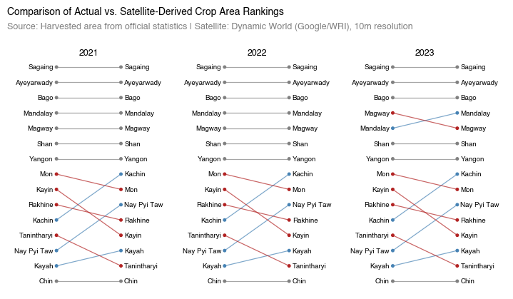
Satellite-Derived vs. Official Harvested Area Comparison#
The table below compares the satellite-derived cropland area estimates with official harvested area statistics in 2023. Compared to the official harvested area, the cropland area derived from satellite data is significantly lower, with the highest difference observed in Tanintharyi region.
| Admin Level 1 | year | Actual Harvested Area (acres) | Satellite-derived Crop Area (acres) | Actual Rank | Satellite-derived Rank | Percent Difference (%) | |
|---|---|---|---|---|---|---|---|
| 0 | Sagaing | 2023 | 15,737,204 | 3,962,762 | 1 | 1 | -297.13% |
| 1 | Ayeyarwady | 2023 | 15,600,272 | 3,029,523 | 2 | 2 | -414.94% |
| 2 | Bago | 2023 | 13,694,134 | 2,708,850 | 3 | 3 | -405.53% |
| 3 | Mandalay | 2023 | 9,080,864 | 2,645,312 | 5 | 4 | -243.28% |
| 4 | Magway | 2023 | 9,900,750 | 2,461,605 | 4 | 5 | -302.21% |
| 5 | Shan | 2023 | 7,783,626 | 1,762,997 | 6 | 6 | -341.50% |
| 6 | Yangon | 2023 | 4,259,410 | 1,120,116 | 7 | 7 | -280.26% |
| 7 | Kachin | 2023 | 1,905,864 | 588,800 | 11 | 8 | -223.69% |
| 8 | Mon | 2023 | 2,896,838 | 371,377 | 8 | 9 | -680.03% |
| 9 | Nay Pyi Taw | 2023 | 937,660 | 346,262 | 13 | 10 | -170.80% |
| 10 | Rakhine | 2023 | 2,647,330 | 320,716 | 10 | 11 | -725.44% |
| 11 | Kayin | 2023 | 2,737,796 | 188,712 | 9 | 12 | -1350.78% |
| 12 | Kayah | 2023 | 445,018 | 65,761 | 14 | 13 | -576.72% |
| 13 | Tanintharyi | 2023 | 1,608,060 | 36,513 | 12 | 14 | -4304.06% |
| 14 | Chin | 2023 | 272,288 | 24,694 | 15 | 15 | -1002.64% |
When comparing regions based on cropland area rankings, the official harvested area data and satellite-based crop area demonstrate comparable patterns, particularly in the Sagaing, Ayeyarwady, and Bago regions. However, for regions with limited cropland area, the two datasets tend to diverge more noticeably.
Crop Seasonality#
Using this time series dataset of EVI images, we apply several pre-processing steps to extract critical phenological parameters: start of season (SOS), middle of season (MOS), end of season (EOS), length of season (LOS), etc. This workflow is heavily inspired by the TIMESAT software.
Pre-processing steps
Remove outliers from dataset on per-pixel basis using median method: outlier if median from a moving window < or > standard deviation of time-series times 2.
Interpolate missing values linearly
Smooth data on per-pixel basis (using Savitsky Golay filter, window length of 3, and polyorder of 1)
Phenology Process
We then extract crop seasonality metrics using the seasonal amplitude method from the phenolopy package.
The chart below shows the result of this process for a single crop pixel. The blue dots represent the raw EVI values, the black line represents the processed EVI values, and the dotted lines represent season parameters extracted for that pixel: start of season, peak of season, and end of season.
Based on the phenology process, we identified the seasonality to start in July and end in February with the peak being in October. This can vary with geographic region and crop type as well, however, that has not been taken into consideration in this version.
EVI and Agricultural GDP#
In this section, we explore the relationship between EVI and agricultural GDP at national and regional levels. We employ regression analysis to quantify the strength and significance of these relationships. We also visualize the temporal trends of EVI and agricultural GDP to assess their alignment over time.
National Level Regression Analysis#
The regression results demonstrate a strong and robust relationship between lagged EVI and agricultural GDP across all model specifications. Lagged EVI (one quarter ago) consistently emerges as the most important predictor of agricultural GDP, showing high statistical significance (p < 0.01) and stable coefficients across all models that include it (Models 2-4). In the full specification model (model 4), the lagged EVI coefficient can be interpreted as: comparing two observations that differ by 1% in lagged EVI, the model predicts on average a difference of 1.15% in agricultural GDP, holding other variables constant.
It is important to note that an alternative specification including rainfall was tested but suffered from severe multicollinearity with EVI measures. The high correlation is expected given that rainfall is a primary driver of vegetation greenness, leading to inflated standard errors and unstable coefficient estimates.
In summary, it was seen that 1% increase in EVI from the last quarter could result in a 1.15% increase in GDP while accountign fopr the changes in nighttime lights, in crop season (July-Feb). Severe changes in rainfall will likely impact this given it directly affects the health of a crop.
It must also be noted that EVI, Nighttime Lights and crop season alone are insufficient to nowcast agricultural GDP, only the positive relationship between the two variables can be suggested.
| Dependent variable: gdp_log | |||||
| Model 1 | Model 2 | Model 3 | Model 4 | Model 5 | |
| (1) | (2) | (3) | (4) | (5) | |
| EVI (log) | 1.701*** | 1.574*** | 1.173*** | -0.396*** | -0.428** |
| (0.447) | (0.332) | (0.311) | (0.147) | (0.188) | |
| NTL Sum (log) | -0.937*** | -0.540*** | -0.388*** | ||
| (0.220) | (0.086) | (0.054) | |||
| EVI 1 Quarter Ago (log) | 2.414*** | 2.334*** | 1.115*** | -0.327* | |
| (0.321) | (0.299) | (0.132) | (0.189) | ||
| Is Crop Season | 1.484*** | ||||
| (0.086) | |||||
| Q2 (Jul-Sep) | -2.066*** | ||||
| (0.084) | |||||
| Q3 (Oct-Dec) | -0.709*** | ||||
| (0.127) | |||||
| Q4 (Jan-Mar) | 0.083 | ||||
| (0.089) | |||||
| Observations | 60 | 59 | 53 | 53 | 53 |
| R2 | 0.200 | 0.591 | 0.705 | 0.959 | 0.986 |
| Adjusted R2 | 0.186 | 0.576 | 0.687 | 0.956 | 0.985 |
| Residual Std. Error | 0.749 (df=58) | 0.536 (df=56) | 0.466 (df=49) | 0.175 (df=48) | 0.103 (df=46) |
| F Statistic | 14.463*** (df=1; 58) | 40.380*** (df=2; 56) | 39.098*** (df=3; 49) | 283.828*** (df=4; 48) | 554.476*** (df=6; 46) |
| Note: | *p<0.1; **p<0.05; ***p<0.01 | ||||
The figure below shows the visualize the coefficient estimates and its uncertainty. The coefficient of interest, EVI 1 Quarter Ago (log), has a 95% confidence interval of 0.849 to 1.380, indicating a strong and statistically significant positive relationship with agricultural GDP.
Show code cell outputs
Temporal Trends at National Level#
The figure below shows agricultural GDP from 2010 to 2024 and quarterly EVI (lagged one quarter) from 2010 to mid 2025. The near-identical cyclical patterns suggest agricultural GDP materializes approximately one quarter later.
When these variables are aggregated at the annual level, the trends between EVI and agricultural GDP remain consistent, except after the year 2020 where agricultural GDP shows a sharper decline compared to EVI. This divergence may be attributed to external economic shocks, such as the COVID-19 pandemic and political instability, which affected the agricultural sector beyond what is captured by vegetation health alone.
It is seen here that the median EVI in July-Sep 2025 which is the beginning of the crop season is higher in 2025 than 2024. The main crop season data for October is incomplete for 2025 at the time of writing.
EVI Changes in 2024 and 2025#
When we zoom in on the year of 2024 and 2025 and compare the annual median EVI during the early crop growing season (July to October), it appears that the EVI values for 2025 are higher than 2024. This may suggest a potential improvement in vegetation health and crop conditions in 2025 compared to the previous year. However, this observation should be interpreted with caution, as the EVI for 2025 only includes data up to early October, and the full growing season data is not yet available. Further monitoring and analysis will be necessary to confirm whether this trend continues through the end of the year.
| Year | EVI | |
|---|---|---|
| 0 | 2024 | 0.3594 |
| 1 | 2025 | 0.3868 |
The pattern in the national level EVI is generally consistent across regions. The table below shows the comparison of median EVI in 2024 and 2025 during the early crop growing season (July to October) across different regions/states in Myanmar. Most of the regions/states show an increase in EVI from 2024 to 2025, while some regions/states such as Nay Pyi Taw and Rakhine show a slight decrease. But as suggested earlier, the 2025 data only covers up to early October, so these observations should be interpreted with caution until the full season data is available.
| Admin Level 1 | EVI 2024 | EVI 2025 | Difference (2025 - 2024) | Percent Difference (%) | |
|---|---|---|---|---|---|
| 0 | Yangon | 0.3096 | 0.3759 | 0.0664 | 21.41 |
| 1 | Shan (East) | 0.4541 | 0.5119 | 0.0578 | 12.73 |
| 2 | Mandalay | 0.3359 | 0.3868 | 0.0508 | 15.15 |
| 3 | Kayin | 0.1563 | 0.1955 | 0.0392 | 25.08 |
| 4 | Shan (South) | 0.4033 | 0.4297 | 0.0264 | 6.55 |
| 5 | Magway | 0.3516 | 0.3750 | 0.0234 | 6.66 |
| 6 | Bago (East) | 0.3321 | 0.3554 | 0.0234 | 7.02 |
| 7 | Kayah | 0.3992 | 0.4218 | 0.0226 | 5.66 |
| 8 | Sagaing | 0.3594 | 0.3789 | 0.0195 | 5.43 |
| 9 | Shan (North) | 0.4727 | 0.4882 | 0.0155 | 3.28 |
| 10 | Kachin | 0.4542 | 0.4647 | 0.0105 | 2.31 |
| 11 | Bago (West) | 0.4140 | 0.4219 | 0.0078 | 1.91 |
| 12 | Nay Pyi Taw | 0.4326 | 0.4307 | -0.0018 | -0.44 |
| 13 | Rakhine | 0.4257 | 0.4218 | -0.0040 | -0.92 |
| 14 | Chin | 0.4669 | 0.4591 | -0.0079 | -1.67 |
| 15 | Tanintharyi | 0.4765 | 0.4606 | -0.0159 | -3.34 |
| 16 | Mon | 0.3674 | 0.3507 | -0.0166 | -4.55 |
| 17 | Ayeyarwady | 0.2460 | 0.2227 | -0.0233 | -9.47 |
State-level EVI and Agricultural GDP#
To further validate the findings from the national level regression analysis, we conduct a sensitivity analysis at the state/region level. This involves replicating the regression models using state-level EVI and agricultural GDP data to examine whether the observed relationships hold true across different geographic scales.
The state-level results largely confirm the national-level findings, with lagged EVI remaining a strong and statistically significant predictor of agricultural GDP.
The first 3 models (Models 1-3) \(R^2\) values are relatively low, indicating that these specifications explain only a small portion of the variation in agricultural GDP at the state level. However, as additional controls are introduced in Models 4 and 5, the explanatory power increases substantially, particularly when state fixed effects are included in Model 5 (\(R^2\) = 0.963).
In model 4, after including the crop season indicator, lagged EVI becomes statistically insignificant, which contrasts with the national-level results where lagged EVI remains significant. This discrepancy may be due to regional heterogeneity in crop seasonality, as different states have varying crop calendars and planting patterns. The uniform application of a single binary crop season indicator across all regions may lead to misspecification, absorbing temporal variation in some regions while failing to capture it accurately in others.
However, the inclusion of state fixed effects in Model 5 addresses these concerns. This specification achieves the highest explanatory power (\(R^2\) = 0.963) and reveals that lagged EVI remains positive and highly significant even after accounting for state-specific characteristics and seasonal patterns. The magnitude is smaller than at the national level, which is expected given that state-level variation is partially absorbed by the fixed effects.
| Dependent variable: gdp_log | ||||||
| Model 1 | Model 2 | Model 3 | Model 4 | Model 5 | Model 6 | |
| (1) | (2) | (3) | (4) | (5) | (6) | |
| Intercept | 11.544*** | 12.278*** | 11.503*** | 6.822*** | 13.923*** | 14.934*** |
| (0.176) | (0.227) | (0.466) | (0.405) | (0.174) | (0.105) | |
| EVI (log) | 0.097 | -0.053 | 0.028 | -1.056*** | -0.245*** | -0.020 |
| (0.137) | (0.139) | (0.148) | (0.122) | (0.036) | (0.026) | |
| EVI 1 Quarter Ago (log) | 0.722*** | 0.837*** | -0.099 | 0.673*** | -0.003 | |
| (0.138) | (0.148) | (0.120) | (0.035) | (0.026) | ||
| Is Crop Season | 2.120*** | 1.602*** | ||||
| (0.084) | (0.024) | |||||
| NTL Sum (log) | 0.097** | 0.150*** | -0.175*** | -0.149*** | ||
| (0.045) | (0.035) | (0.016) | (0.010) | |||
| Q2 (Jul-Sep) | -1.938*** | |||||
| (0.016) | ||||||
| Q3 (Oct-Dec) | -0.673*** | |||||
| (0.019) | ||||||
| Q4 (Jan-Mar) | -0.022 | |||||
| (0.016) | ||||||
| Observations | 1057 | 1039 | 937 | 937 | 937 | 937 |
| R2 | 0.000 | 0.026 | 0.035 | 0.425 | 0.963 | 0.987 |
| Adjusted R2 | -0.000 | 0.024 | 0.032 | 0.423 | 0.962 | 0.987 |
| Residual Std. Error | 1.264 (df=1055) | 1.246 (df=1036) | 1.250 (df=933) | 0.965 (df=932) | 0.248 (df=915) | 0.145 (df=913) |
| F Statistic | 0.496 (df=1; 1055) | 13.852*** (df=2; 1036) | 11.275*** (df=3; 933) | 172.434*** (df=4; 932) | 1130.127*** (df=21; 915) | 3072.611*** (df=23; 913) |
| Note: | *p<0.1; **p<0.05; ***p<0.01 | |||||
Out-of-Sample Prediction: 2023-2025#
| Quarter | Actual GDP | Predicted GDP | Error | Error (%) | |
|---|---|---|---|---|---|
| 51 | 2023-01-01 | 3551069.13 | 3710228.77 | -159159.64 | -4.48 |
| 52 | 2023-04-01 | 559112.32 | 404122.13 | 154990.19 | 27.72 |
| 53 | 2023-07-01 | 1669657.09 | 1938470.39 | -268813.30 | -16.10 |
| 54 | 2023-10-01 | 3897192.75 | 3434163.12 | 463029.63 | 11.88 |
| 55 | 2024-01-01 | 3693111.89 | 3511943.39 | 181168.50 | 4.91 |
| 56 | 2024-04-01 | 615023.56 | 606755.88 | 8267.68 | 1.34 |
| 57 | 2024-07-01 | 1836622.80 | 1697645.28 | 138977.51 | 7.57 |
| 58 | 2024-10-01 | 3624389.26 | 3556715.90 | 67673.35 | 1.87 |
| 59 | 2025-01-01 | 3434594.06 | 5389431.08 | -1954837.02 | -56.92 |
Lastly, we evaluate the model’s predictive performance for the years 2023 to 2025, which were not included in the training dataset. The model demonstrates strong predictive accuracy, with predicted agricultural GDP values closely aligning with observed figures for 2023 and 2024. However, the model prediction on Q1 2025 diverges from expectations, potentially due to unforeseen factors affecting agricultural productivity that are not captured by EVI alone.
Conclusion#
The analysis demonstrates a robust relationship between lagged EVI and agricultural GDP at both national and regional levels. Lagged EVI consistently emerges as a significant predictor of agricultural GDP. However, it is important to note that while EVI effectively reflects vegetation health and crop conditions, and its predictive power on crop yield is evident, it does not capture the full complexity of agricultural GDP. Furthermore, the the predictive relationship observed in historical data may not hold under changing conditions, such as ongoing political and economic transitions, natural disasters, climate variability and extreme weather events.
base = alt.Chart(
    evi_gdp_annual.assign(
        evi_log_std=(evi_gdp_annual["evi"] - evi_gdp_annual["evi"].mean())
        / evi_gdp_annual["evi"].std(),
        gdp_log_std=(evi_gdp_annual["gdp_lag_1"] - evi_gdp_annual["gdp_lag_1"].mean())
        / evi_gdp_annual["gdp_lag_1"].std(),
    ).melt(
        id_vars="date",
        value_vars=["evi_log_std", "gdp_log_std"],
        var_name="indicator",
    )
)

base.mark_line().encode(
    x=alt.X("date:T", title="Date"),
    y=alt.Y("value:Q", scale=alt.Scale(zero=False), title="Standardized Log of EVI"),
    color=alt.Color("indicator:N", title="Indicator"),
).properties(width=600, height=300, title="EVI Over Time")
References#
- AJL17
George Azzari, Meha Jain, and David B. Lobell. Towards fine resolution global maps of crop yields: Testing multiple methods and satellites in three countries. Remote Sensing of Environment, 202:129–141, December 2017. doi:10.1016/j.rse.2017.04.014.
- BRVLJ10
I. Becker-Reshef, E. Vermote, M. Lindeman, and C. Justice. A generalized regression-based model for forecasting winter wheat yields in Kansas and Ukraine using MODIS data. Remote Sensing of Environment, 114(6):1312–1323, June 2010. doi:10.1016/j.rse.2010.01.010.
- BF13
Douglas K. Bolton and Mark A. Friedl. Forecasting crop yield using remotely sensed vegetation indices and crop phenology metrics. Agricultural and Forest Meteorology, 173:74–84, May 2013. doi:10.1016/j.agrformet.2013.01.007.
- DMCS03
Paul C. Doraiswamy, Sophie Moulin, Paul W. Cook, and Alan Stern. Crop Yield Assessment from Remote Sensing. Photogrammetric Engineering & Remote Sensing, 69(6):665–674, June 2003. doi:10.14358/PERS.69.6.665.
- HDM+02(1,2)
A Huete, K Didan, T Miura, E.P Rodriguez, X Gao, and L.G Ferreira. Overview of the radiometric and biophysical performance of the MODIS vegetation indices. Remote Sensing of Environment, 83(1-2):195–213, November 2002. doi:10.1016/S0034-4257(02)00096-2.
- JA15
Hadi H. Jaafar and Farah A. Ahmad. Crop yield prediction from remotely sensed vegetation indices and primary productivity in arid and semi-arid lands. International Journal of Remote Sensing, 36(18):4570–4589, September 2015. doi:10.1080/01431161.2015.1084434.
- JPZ+22
Zhonglin Ji, Yaozhong Pan, Xiufang Zhu, Dujuan Zhang, and Jinyun Wang. A generalized model to predict large-scale crop yields integrating satellite-based vegetation index time series and phenology metrics. Ecological Indicators, 137:108759, April 2022. doi:10.1016/j.ecolind.2022.108759.
- Joh16(1,2,3,4)
David M. Johnson. A comprehensive assessment of the correlations between field crop yields and commonly used MODIS products. International Journal of Applied Earth Observation and Geoinformation, 52:65–81, October 2016. doi:10.1016/j.jag.2016.05.010.
- JLH+18
František Jurečka, Vojtěch Lukas, Petr Hlavinka, Daniela Semerádová, Zdeněk Žalud, and Miroslav Trnka. Estimating Crop Yields at the Field Level Using Landsat and MODIS Products. Acta Universitatis Agriculturae et Silviculturae Mendelianae Brunensis, 66(5):1141–1150, October 2018. doi:10.11118/actaun201866051141.
- KMC20(1,2,3,4)
Kefyalew Sahle Kibret, Carsten Marohn, and Georg Cadisch. Use of MODIS EVI to map crop phenology, identify cropping systems, detect land use change and drought risk in Ethiopia – an application of Google Earth Engine. European Journal of Remote Sensing, 53(1):176–191, January 2020. doi:10.1080/22797254.2020.1786466.
- Pet18
Lillian Kay Petersen. Real-Time Prediction of Crop Yields From MODIS Relative Vegetation Health: A Continent-Wide Analysis of Africa. Remote Sensing, 10(11):1726, November 2018. Number: 11 Publisher: Multidisciplinary Digital Publishing Institute. doi:10.3390/rs10111726.
- PAK+22
Hoa Thi Pham, Joseph Awange, Michael Kuhn, Binh Van Nguyen, and Luyen K. Bui. Enhancing Crop Yield Prediction Utilizing Machine Learning on Satellite-Based Vegetation Health Indices. Sensors, 22(3):719, January 2022. doi:10.3390/s22030719.
- RRK+09
Atiqur Rahman, Leonid Roytman, Nir Y. Krakauer, Mohammad Nizamuddin, and Mitch Goldberg. Use of Vegetation Health Data for Estimation of Aus Rice Yield in Bangladesh. Sensors, 9(4):2968–2975, April 2009. doi:10.3390/s90402968.
- SH15
Jingjing Shi and Jingfeng Huang. Monitoring Spatio-Temporal Distribution of Rice Planting Area in the Yangtze River Delta Region Using MODIS Images. Remote Sensing, 7(7):8883–8905, July 2015. doi:10.3390/rs70708883.
- SCC+13(1,2,3)
N. T. Son, C. F. Chen, C. R. Chen, L. Y. Chang, H. N. Duc, and L. D. Nguyen. Prediction of rice crop yield using MODIS EVI−LAI data in the Mekong Delta, Vietnam. International Journal of Remote Sensing, 34(20):7275–7292, October 2013. doi:10.1080/01431161.2013.818258.
- TMA+23
Gizachew Ayalew Tiruneh, Derege Tsegaye Meshesha, Enyew Adgo, Atsushi Tsunekawa, Nigussie Haregeweyn, Ayele Almaw Fenta, Tiringo Yilak Alemayehu, Temesgen Mulualem, Genetu Fekadu, Simeneh Demissie, and José Miguel Reichert. Mapping crop yield spatial variability using Sentinel-2 vegetation indices in Ethiopia. Arabian Journal of Geosciences, 16(11):631, November 2023. doi:10.1007/s12517-023-11754-x.
- WDS15
J. S. J. Wijesingha, N. L. Deshapriya, and L. Samarakoon. Rice Crop Monitoring and Yield Assessment with MODIS 250m Gridded Vegetation Products: A Case Study of Sa Kaeo Province, Thailand. The International Archives of the Photogrammetry, Remote Sensing and Spatial Information Sciences, XL-7/W3:121–127, April 2015. doi:10.5194/isprsarchives-XL-7-W3-121-2015.
- WZZ+23
Bingfang Wu, Miao Zhang, Hongwei Zeng, Fuyou Tian, Andries B Potgieter, Xingli Qin, Nana Yan, Sheng Chang, Yan Zhao, Qinghan Dong, Vijendra Boken, Dmitry Plotnikov, Huadong Guo, Fangming Wu, Hang Zhao, Bart Deronde, Laurent Tits, and Evgeny Loupian. Challenges and opportunities in remote sensing-based crop monitoring: a review. National Science Review, 10(4):nwac290, March 2023. doi:10.1093/nsr/nwac290.