Estimating Activity Using Mobility Data

Understanding population movement can provide valuable insights for public policy and disaster response efforts, particularly during crises when less movement often correlates with reduced economic activity.

Similar to initiatives such as the COVID-19 Community Mobility Reports, Facebook Population During Crisis, and Mapbox Movement Data, we have developed a range of crisis-relevant indicators. These include baseline and subsequent device densities, as well as metrics like percent change and z-score. These indicators are derived by aggregating device counts within specific geographical tiles and across various time periods, utilizing longitudinal mobility data.

It’s important to note the inherent limitations associated with this approach, as detailed in mobility-activity-limitations. Notably, mobility data is typically collected through convenience sampling methods and lacks the controlled methodology of randomized trials.

Data

In this section, we import from the data sources, available either publicly or via data.

Area of Interest

In this step, we import the SEZ points and create a buffer of 30 km around them. Later, we do a tessellation with h3 polygons of level 6. The resulting tessellation can be explored below.

Make this Notebook Trusted to load map: File -> Trust Notebook

Mobility Data

The WB Data Lab team has acquired longitudinal human mobility data encompassing anonymized timestamped geographical points generated by GPS-enabled devices located in Myanmar. The dataset we are using for this analysis spans across 2020.

The project team has utilized the longitudinal mobility data to derive several key metrics. Specifically, we compute baseline and subsequent device densities, denoted as n_baseline and count respectively, along with metrics such as percent change (percent_change and Z-score (z-score). These indicators are derived by aggregating the device count within each tile and at each time period. The devices are sourced from the longitudinal mobility data. For further details, please refer to the documentation provided in mobility-data and mobility-activity-methodology.

Show code cell source Hide code cell source

len(ddf)

561632137

Spatial Aggregation

The indicators are aggregated spatially on H3 resolution 6 tiles. This is equivalent to approximately to an area of \(36 Km^2\) on average as illustrated below.

Make this Notebook Trusted to load map: File -> Trust Notebook

Temporal Aggregation

The indicators are aggregated daily on the localized date in the Europe/Istanbul (UTC+3) timezone.

Implementation

Calculate ACTIVITY

In this step, we compute ACTIVITY as a density metric. Specifically, we tally the total number of devices detected within each designated area of interest, aggregated on a daily basis. It’s important to highlight that this calculation is based on a spatial join approach, which determines whether a device has been detected within an area of interest at least once. This method, while straightforward, represents a simplified approach compared to more advanced techniques such as estimating stay locations and visits.

Additionally, we create a column weekday that will come handy later on when standardizing.

Calculate BASELINE

In this step, we choose the period spanning January 1, 2020 to February 29, 2020 as the baseline. The baseline is calculated for each tile and for each time period, according to the spatial and temporal aggregations.

In fact, the result are 7 different baselines for each tile. We calculate the mean device density for each tile and for each day of the week (Mon-Sun).

Taking a sneak peek,

Calculate Z-Score and Percent Change

A z-score serves as a statistical metric indicating the deviation of a specific data point from the mean (average) of a given dataset, expressed in terms of standard deviations. It is particularly valuable for standardizing and facilitating meaningful comparisons across various datasets. By evaluating the z-scores, one can gauge the extent to which a dataset diverges from its mean, while accounting for variance. Conversely, a percent change offers a simpler interpretation but lacks the detailed information provided by z-scores.

Creating StandardScaler for each hex_id,

Additionally, we calculate the percent change. While the z-score offers more robustness to outliers and numerical stability, the percent change can be used when interpretability is most important. Thus, preparing columns,

	hex_id	date	count	n_baseline	n_difference	percent_change	z_score	Name
221430	86658935fffffff	2020-02-12	10	3.200000	6.800000	212.500000	2.576855	NaN
80965	86658935fffffff	2020-01-17	11	2.750000	8.250000	300.000000	2.942078	NaN
1490422	86658932fffffff	2020-12-28	8	10.625000	-2.625000	-24.705882	-0.080882	NaN
1477934	86658932fffffff	2020-12-26	3	11.111111	-8.111111	-73.000000	-0.889698	NaN
1467787	86658932fffffff	2020-12-24	14	6.375000	7.625000	119.607843	0.889698	NaN
...	...	...	...	...	...	...	...	...
6114	863c5b28fffffff	2020-01-03	25	37.666667	-12.666667	-33.628319	-0.392411	NaN
3045	863c5b28fffffff	2020-01-02	5	28.555556	-23.555556	-82.490272	-1.245477	NaN
2	863c5b28fffffff	2020-01-01	17	41.777778	-24.777778	-59.308511	-0.733637	NaN
142474	863c5b217ffffff	2020-01-29	12	4.800000	7.200000	150.000000	3.244059	NaN
97151	863c5b217ffffff	2020-01-21	11	3.200000	7.800000	243.750000	2.884559	NaN

526220 rows × 8 columns

Findings

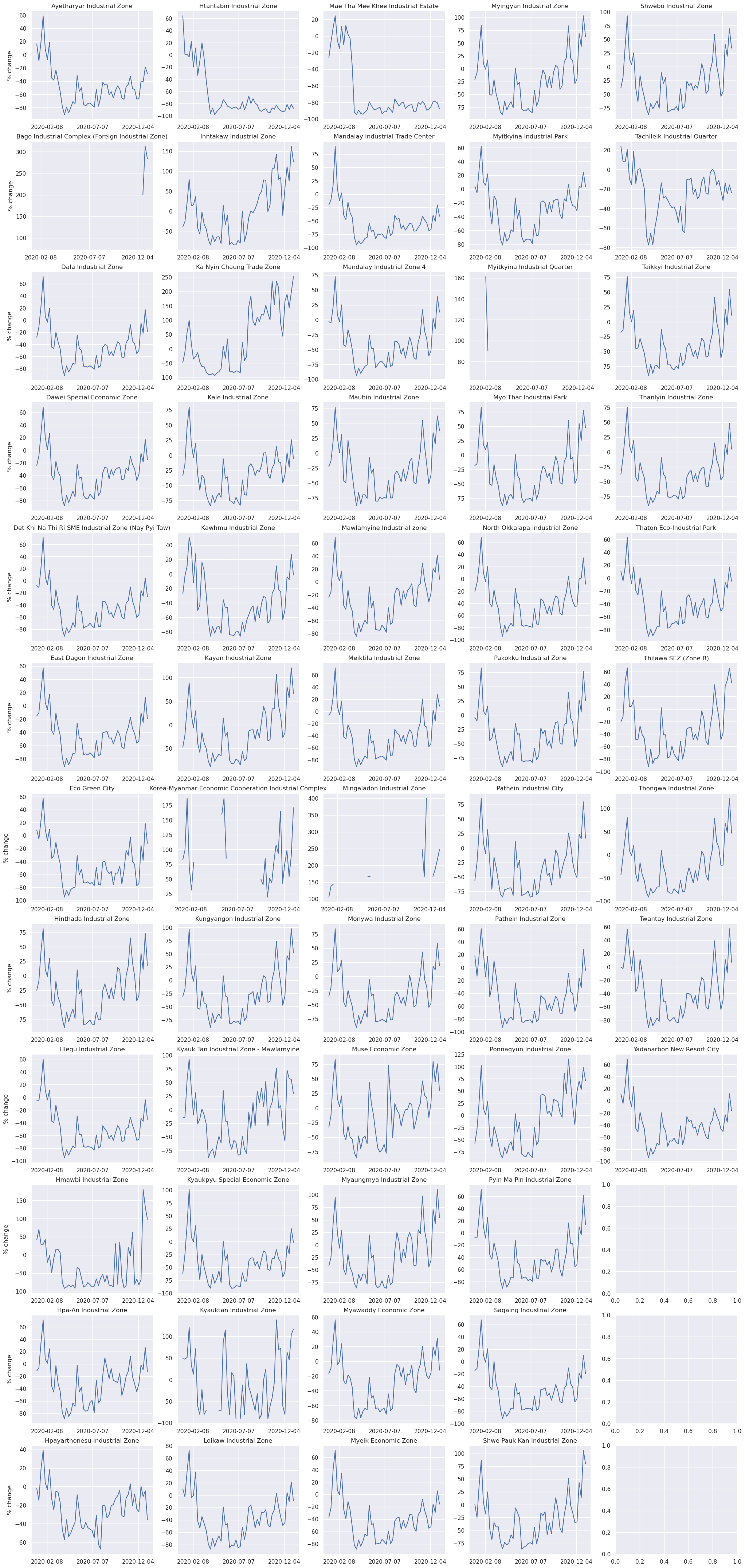
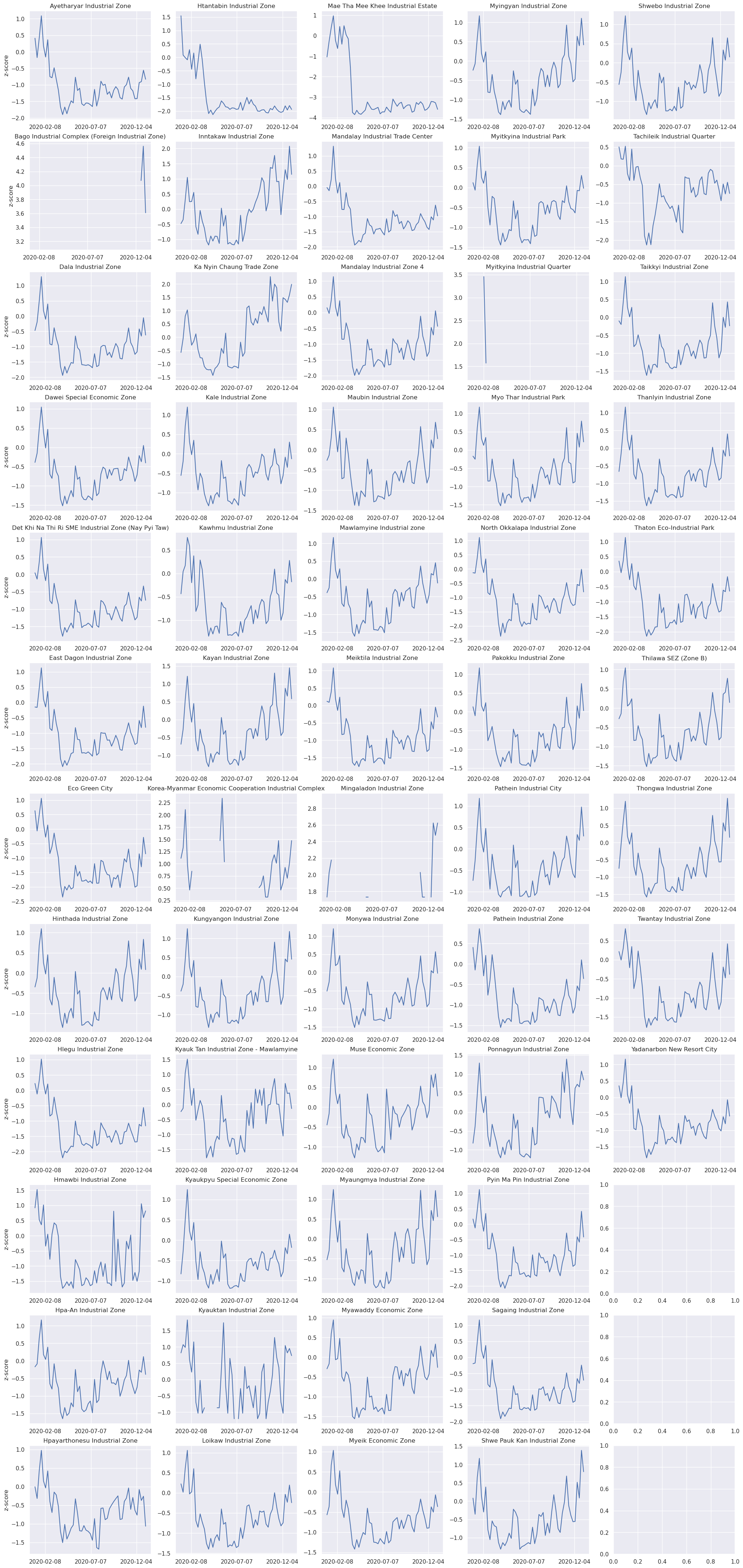
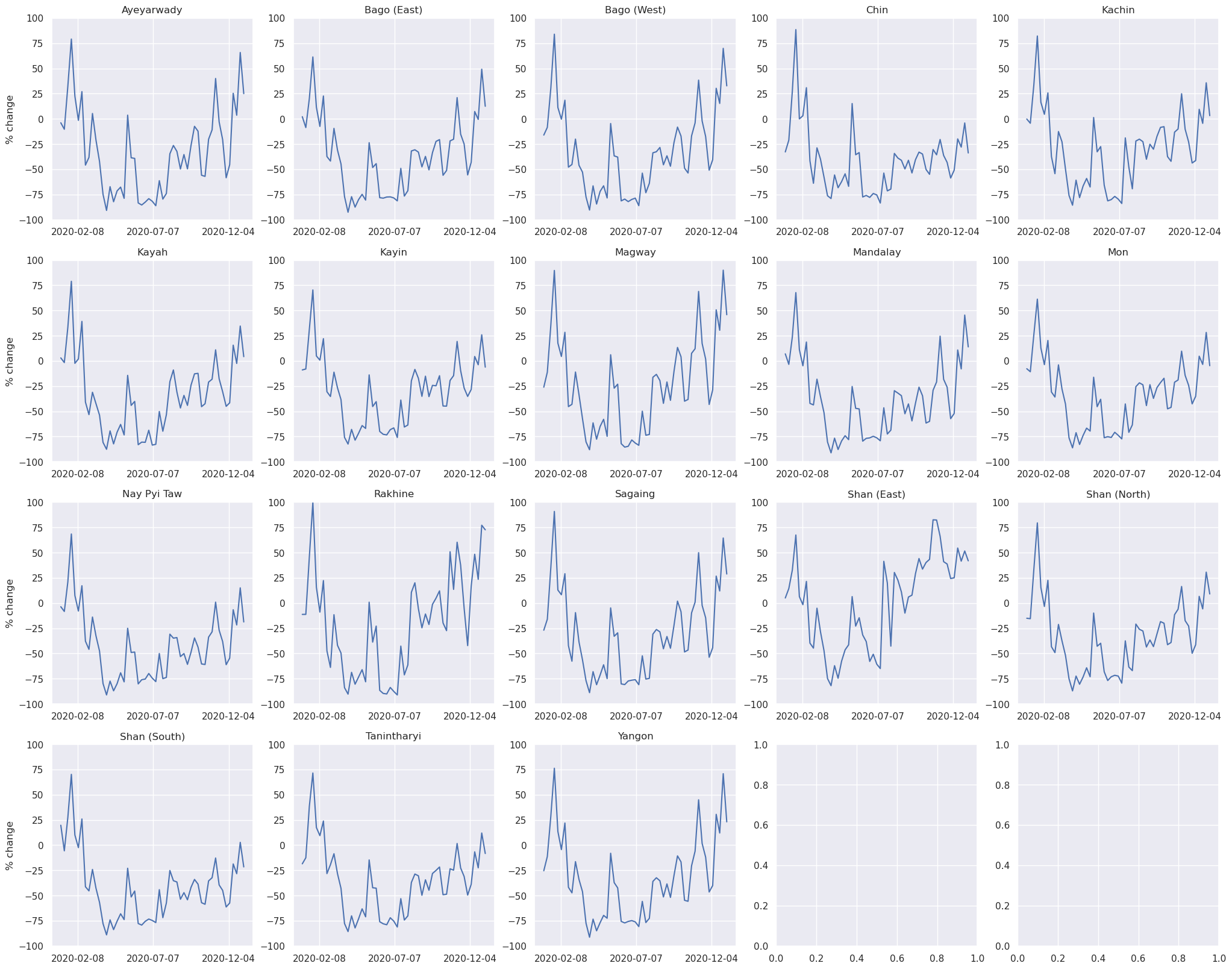
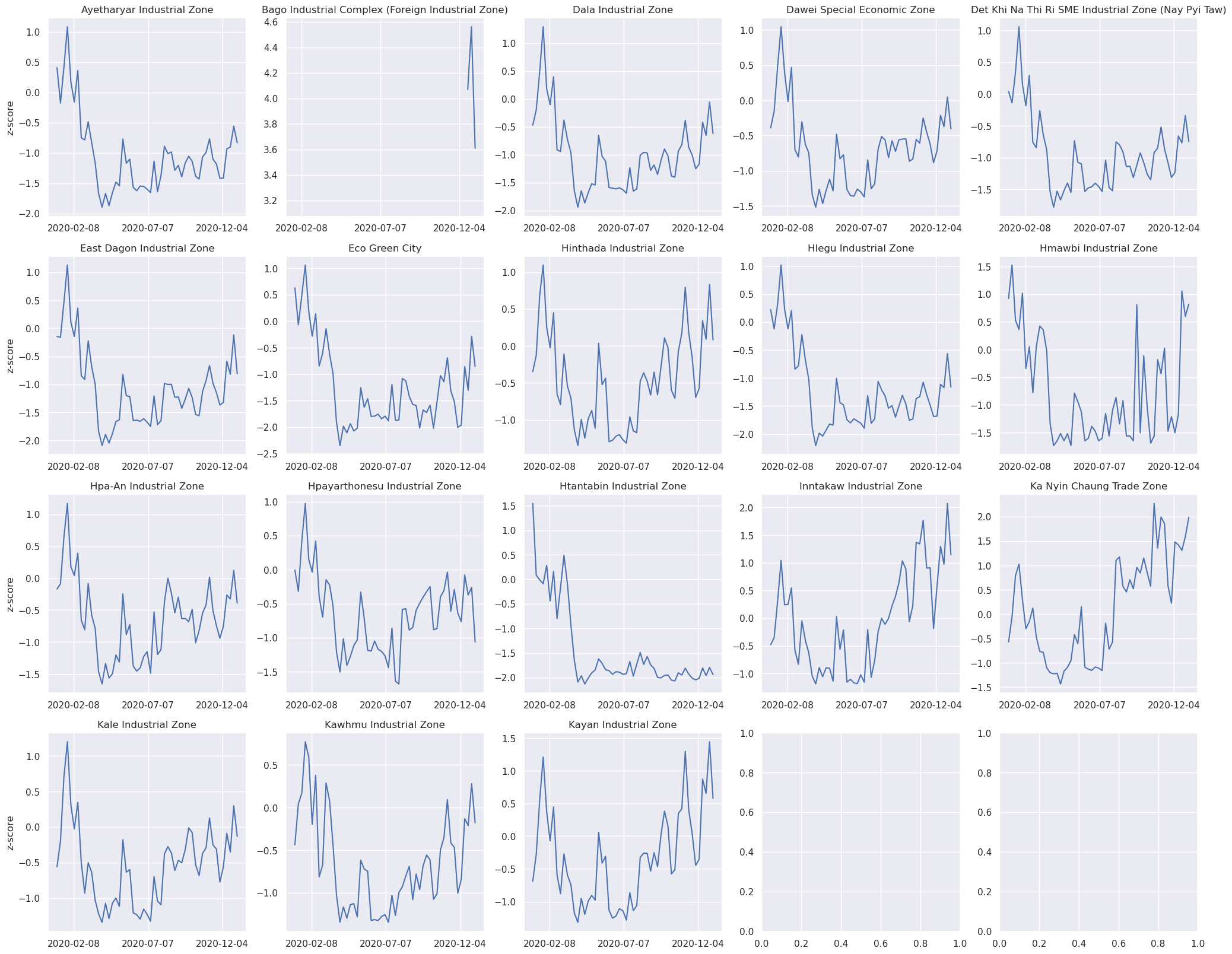
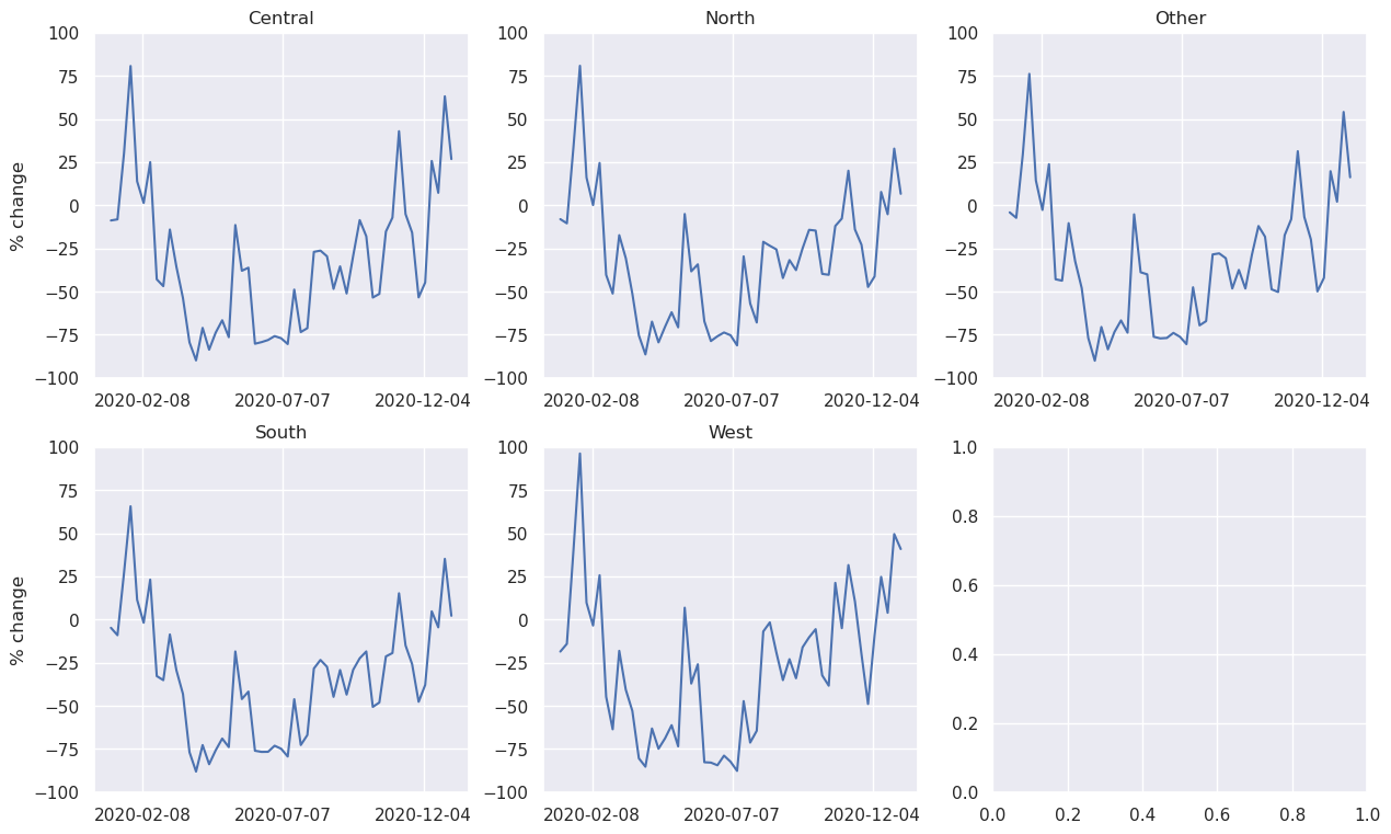
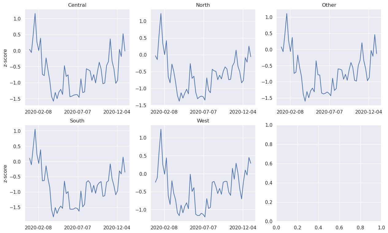
Less movement typically means less economic activity. A potential use of movement “activity” indicators could be to see the their evolution in time and correlatation to other features. We present the results (i.e., percent_change and z_score) on Speial Economic Zones, Administrative 1 boundaries and on the defined Regions.

Aggregation method: Activity index calculated at h3 level 6 was aggregated, first, by averaging the values across the SEZ, Admin 1 or Region, daily. Later, a weekly aggregation was performed.

By Special Economic Zones

Percentage Change

Z-Score

By Admin 1

Percentage Change

Z-Score

By Region

Percentage Change

Z-Score

Limitations

The methodology presented is an exploratory analysis pilot aiming to shed light on the economic situation in Syria and Türkiye leveraging alternative data, especially when we are confronted with the absence of traditional data and methods. Mobility data, like any other type of data, comes with limitations and underlying assumptions that should be considered when interpreting and using the data.

Caution

Here are some common limitations and assumptions associated with mobility data:

Limitations:

• Sampling Bias: Mobility data is primarily collected through convenience sampling and lacks the controlled methodology of randomized trials.

• Selection Bias: Users who opt to share their mobility data may not be representative of the entire population, potentially introducing selection bias.

• Privacy Concerns: The collection of mobility data may raise privacy issues, as it can sometimes be linked to individuals, potentially violating their privacy.

• Data Quality: Data quality can vary, and errors, inaccuracies, or missing data points may be present, which can affect the reliability of analyses.

• Temporal and Spatial Resolution: Mobility data may not capture all movements or may lack fine-grained temporal or spatial resolution, limiting its utility for some applications.

• Lack of Contextual Information: Mobility data primarily captures movement patterns and geolocation information. It may lack other crucial contextual information, such as transactional data, business types, or specific economic activities, which are essential for accurate estimation of economic activity.

• Private Intent Data: The methodology relies on private intent data. In other words, the input data, i.e. the mobility data, was not produced or collected to analyze the population of interest or address the research question as its primary objective but it was repurposed for the public good. The benefits and caveats when using private intent data have been discussed extensively in the World Development Report 2021 .

Assumptions:

• Homogeneity: Mobility data often assumes that the mobility patterns of individuals or groups are relatively consistent over time and space, which may not always be the case.

• Consistency in Data Sources: Mobility data may assume consistency in data sources and methodologies across different regions or datasets, which may not always hold true.

• User Behavior: Assumptions about user behavior, such as the purpose of travel or preferred routes, are often made when interpreting mobility data.

• Implicit Data Interpretation: Interpretation of mobility data often assumes that certain behaviors or patterns observed in the data have a specific meaning, which may not always be accurate without additional context.

• App Usage as a Proxy: In some cases, the use of specific apps or devices may be used as a proxy for mobility data, assuming that it accurately represents individual movements.

It’s important to be aware of these limitations and assumptions when working with mobility data and to consider their potential impact on the conclusions drawn from the data. Additionally, researchers and analysts should explore ways to address these limitations and validate assumptions when conducting mobility data analyses.

See also

For further discussion on limitations and assumptions, please check out the Development Data Partnership Documentation on Mobility Data.

References