Trends in Enhanced Vegetation Index in Bolivia

This notebook presents the analysis of crop productivity trends across Bolivia based on Enhanced Vegetation Index. By leveraging the satellite-derived vegetation indices, we aim to assess how crop yields have changed over time. EVI is specifically designed to optimize the sensitivity to high-biomass regions, reduce atmospheric and soil background noise, and provide a more accurate measure of vegetation health. Because EVI closely tracks photosynthetic activity and green biomass, it serves as a reliable proxy for crop yield.

Data

This analysis utilizes two primary datasets:

• MODIS EVI Data: Sourced from NASA’s Moderate Resolution Imaging Spectroradiometer (MODIS) on the Terra and Aqua satellites, this dataset provides EVI values at a 250-meter spatial resolution, with data collected every 16 days. The analysis focuses on yearly aggregated EVI values from 2014 to 2024.

• Global 30-meter Land Cover (GLC-FCS30D): This dataset offers detailed land cover classifications at a 30-meter resolution, spanning from 1985 to 2022. It is developed using continuous change detection methods and extensive Landsat imagery, providing annual updates and 35 land-cover subcategories.

• Administrative Boundaries: Geographic boundaries for Bolivia are sourced from the GeoBoundaries project. These boundaries are used to spatially aggregate EVI statistics and facilitate reporting at various administrative levels, thus enabling region-specific analysis of crop productivity trends.

Methodology

The analysis follows these main steps:

Cropland Classification Selection

We focus exclusively on cropland areas, using the GLC-FCS30D land cover dataset. Specifically, we select all the following crop types:

• 10: Rainfed cropland

• 11: Herbaceous cover cropland

• 12: Tree or shrub cover cropland

• 20: Irrigated cropland

Masking EVI Data

We created a binary mask for each cropland type and these cropland masks are applied to the EVI data, ensuring that only EVI values corresponding to cropland areas are included in the analysis. This step filters out non-cropland pixels and focuses the analysis on crop productivity.

Crop Seasonality

Using this time series dataset of EVI images, we apply several pre-processing steps to extract critical phenological parameters: start of season (SOS), middle of season (MOS), end of season (EOS), length of season (LOS), etc. This workflow is heavily inspired by the TIMESAT software, although in this implementation we use the Phenolopy open-source package. Below is the steps:

• Remove outliers from dataset on per-pixel basis using median method: outlier if median from a moving window < or > standard deviation of time-series times 2.

• Interpolate missing values linearly

• Smooth data on per-pixel basis (using Savitsky Golay filter, window length of 3, and polyorder of 1)

We then extract crop seasonality metrics using the seasonal amplitude method from the phenolopy package.

Time Series Construction and Zonal Statistics

For each region (as defined by administrative boundaries) and each cropland type, we constructed a time series of EVI values during the growing season. We aggregated the median values for each region and year, and summarizing the EVI trends over time for each cropland class.

Assumptions

In this analysis, we assume that no changes in cropland from 2022 onwards, as the GLC-FCS30D land cover data is only available up to 2022. For years after 2022, the cropland mask from 2022 is used.

Insights

Growing season

The chart below shows the result of this process for a single crop pixel. The green dots represent the raw EVI values, the black line represents the processed EVI values, and the red dotted lines represent season parameters extracted for that pixel: start of season, peak of season, and end of season.

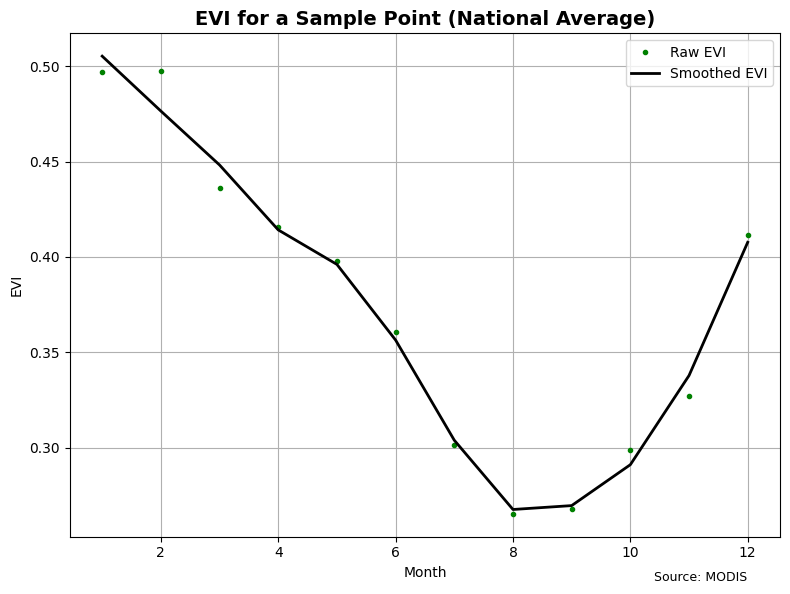
Based on the phenology process, we identified the seasonality to start in October/November and end in March/April with the peak being in January. This can vary with geographic region and crop type as well, however, that has not been taken into consideration in this version.

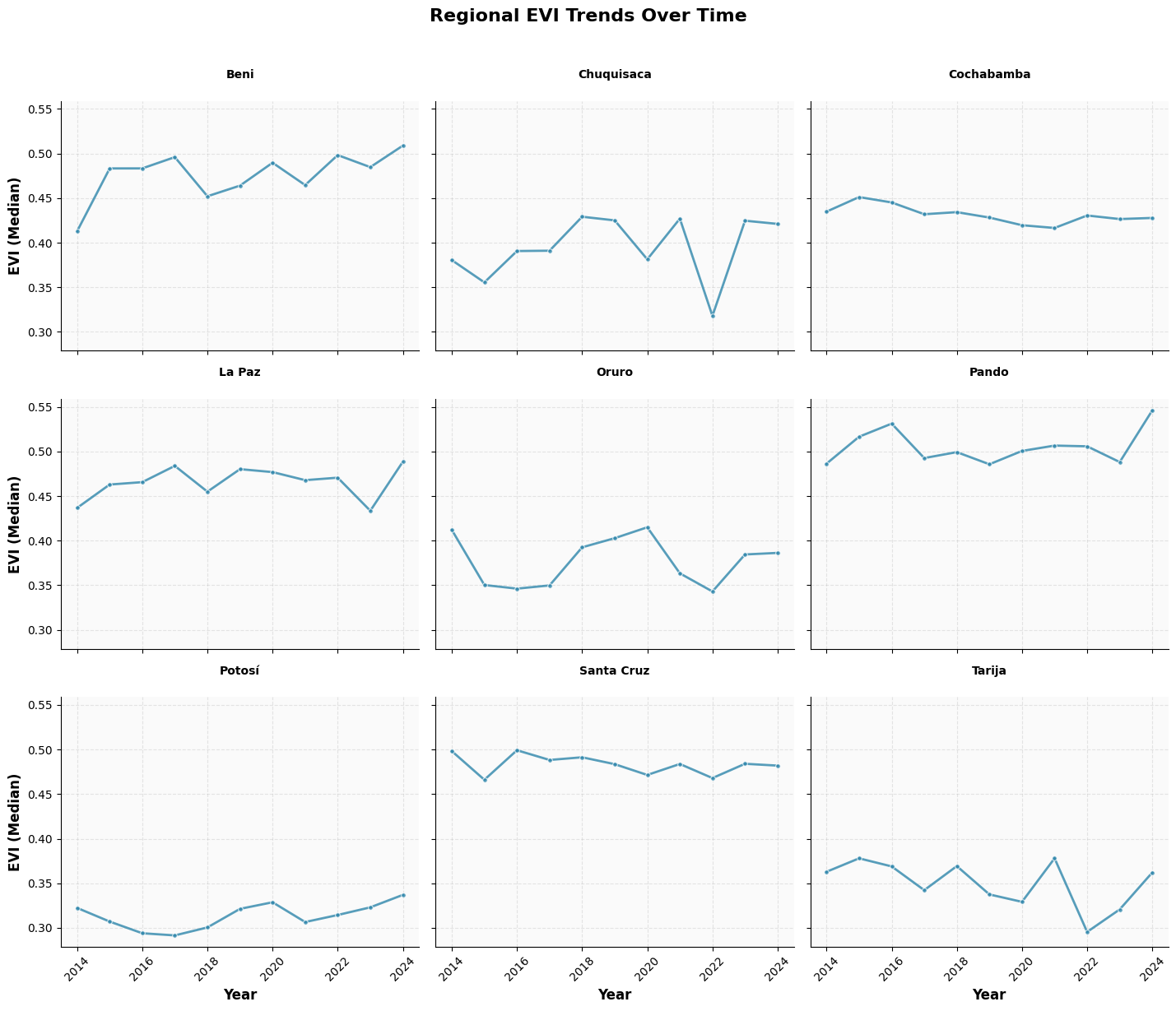
EVI Trend over years across regions

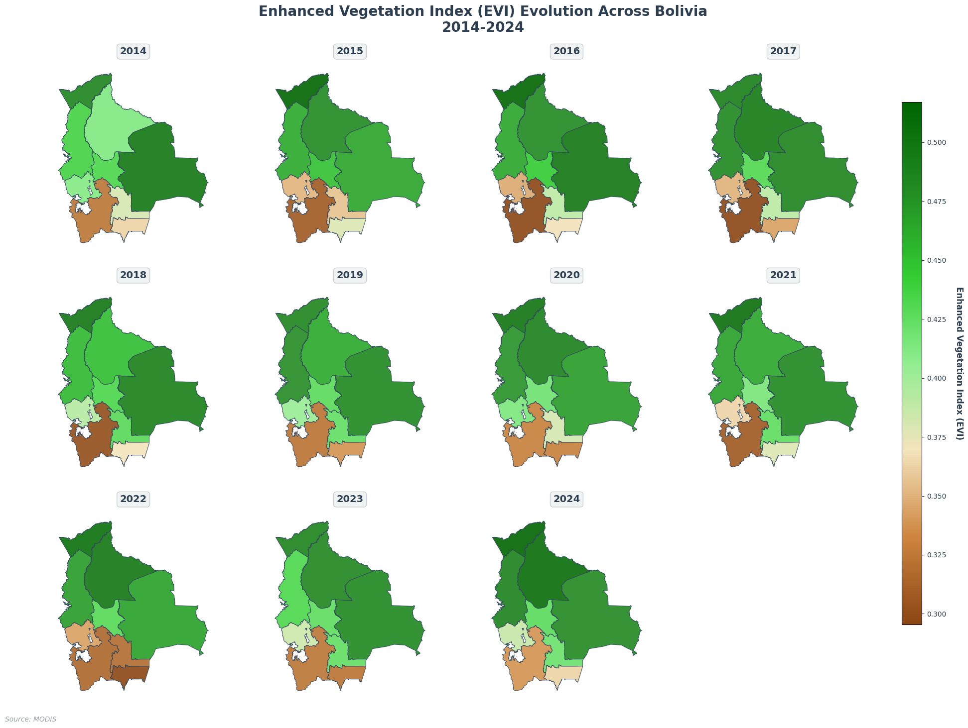
The figure below displays Enhanced Vegetation Index (EVI) trends from 2014 to 2024 across Bolivia’s nine administrative regions.

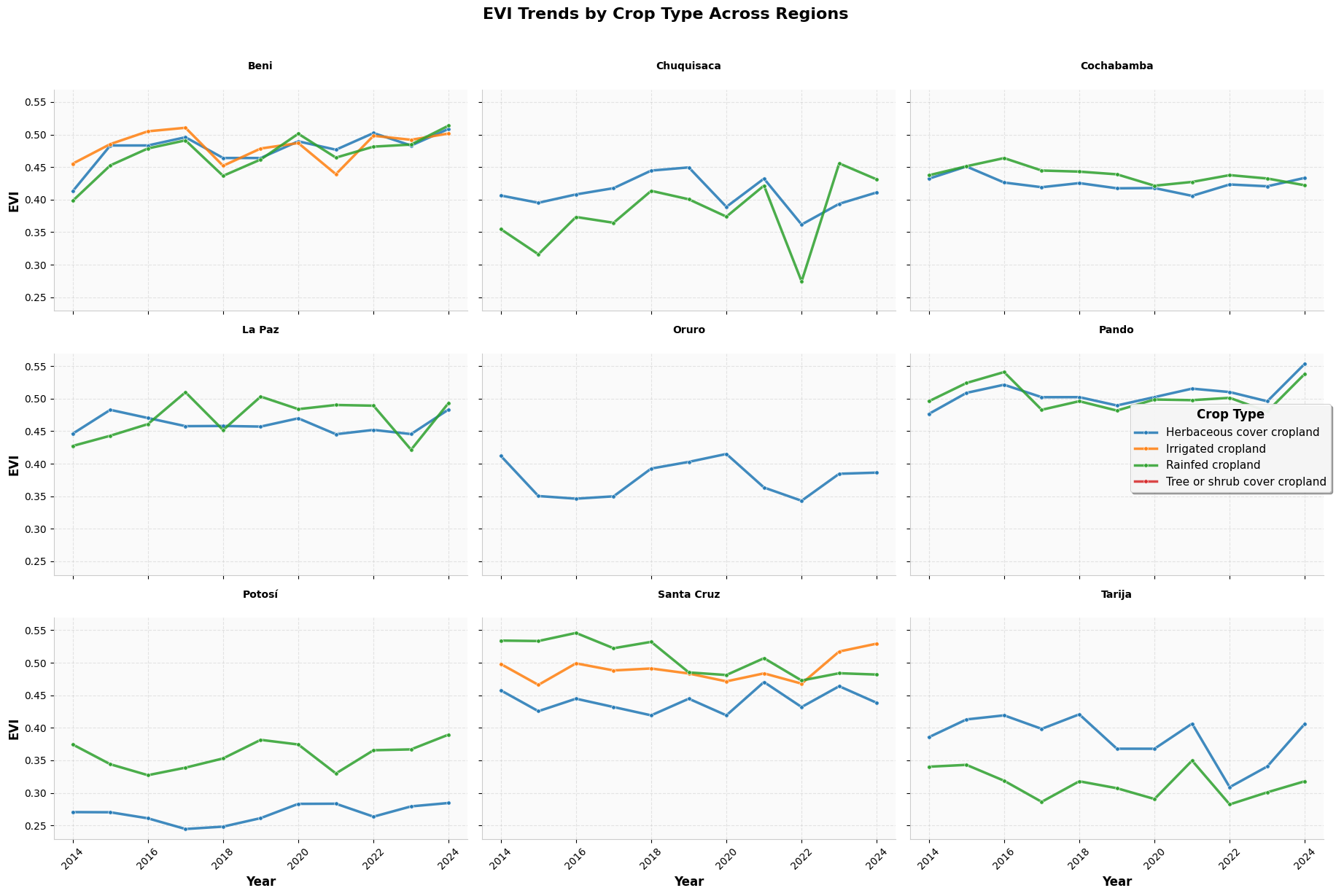
EVI Trend over years across regions and crop types

The figure below displays Enhanced Vegetation Index (EVI) trends from 2014 to 2024 across Bolivia’s nine administrative regions, segmented by four different cropland types.

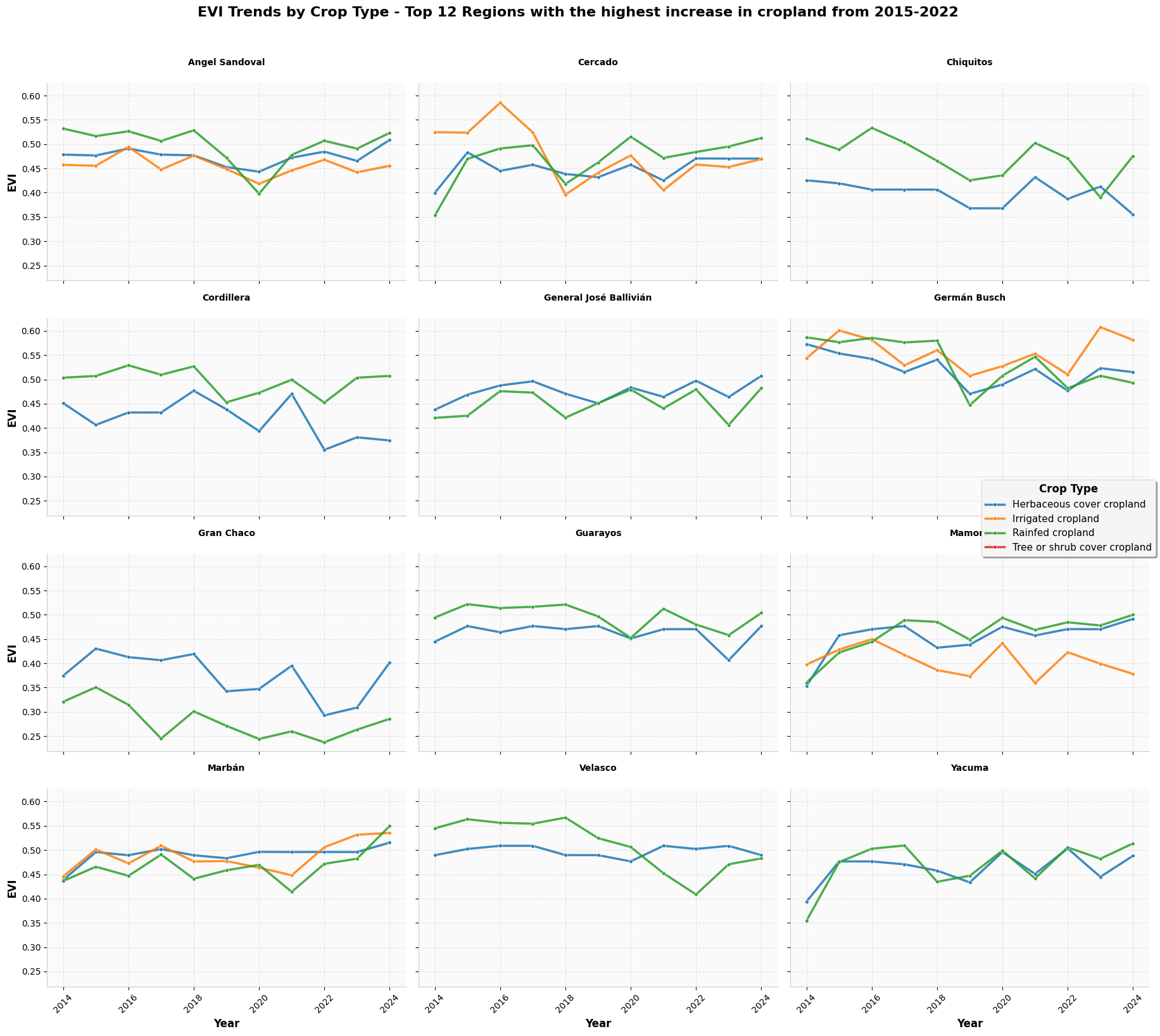
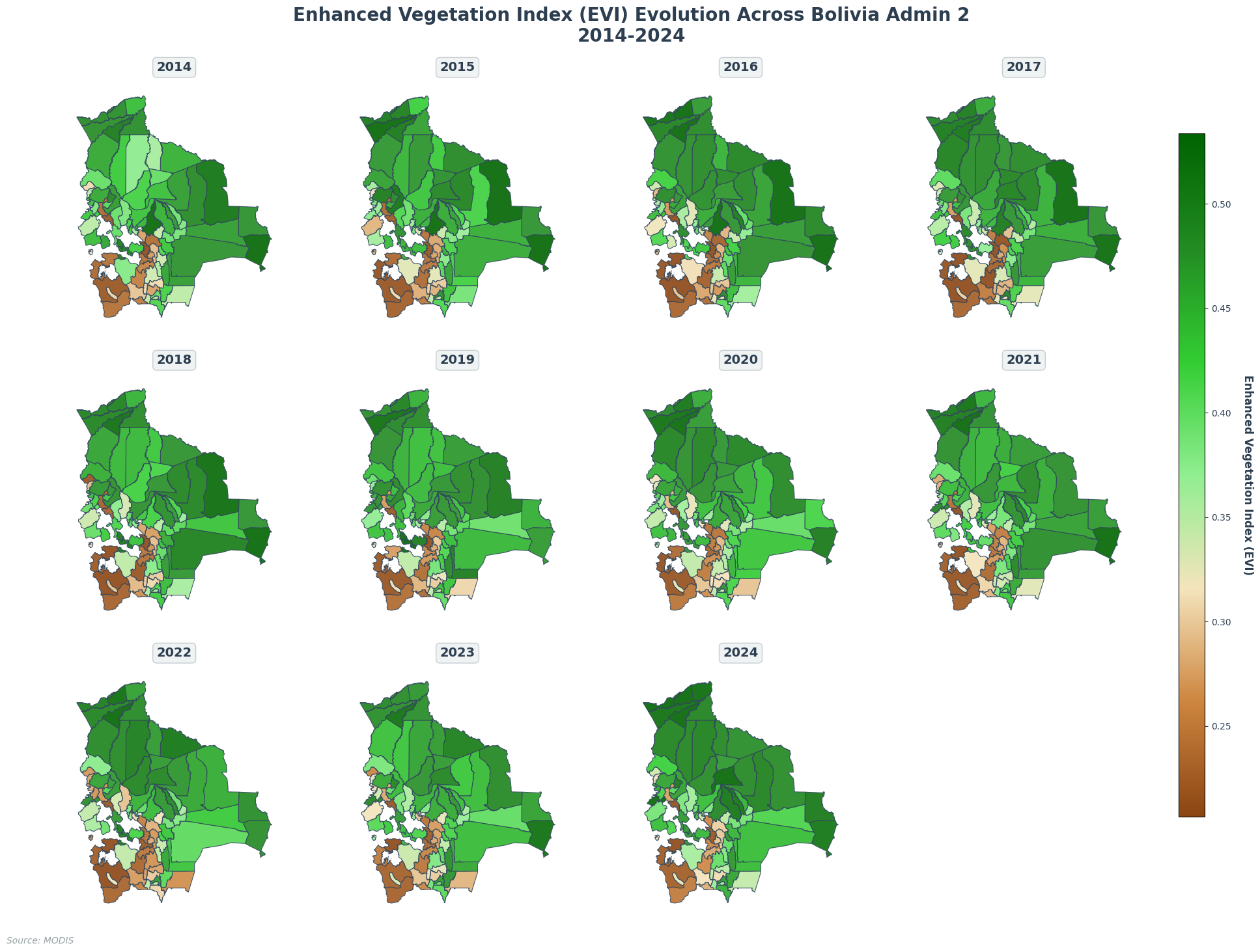
The figure below displays Enhanced Vegetation Index (EVI) trends from 2014 to 2024 across top 10 level 2 administrative regions, segmented by four different cropland types.

This figure displays maps illustrating how EVI changed in each region annually.

Crop land Area

The table below shows top 10 region with the highest absolute percentage change compared between 2015 and 2022.

	Region	Crop Area 2015 (ha)	Crop Area 2022 (ha)	Percentage Change (%)	Absolute Percentage Change (%)
0	Ingavi	265.77	780.57	193.70	193.70
1	Los Andes	963.36	2114.01	119.44	119.44
2	Abel Iturralde	2320.56	4896.27	111.00	111.00
3	Velasco	192131.91	398822.40	107.58	107.58
4	Omasuyos	326.34	590.13	80.83	80.83
5	Moxos	8680.86	15600.87	79.72	79.72
6	Germán Busch	74953.35	132511.77	76.79	76.79
7	Marbán	42757.02	72476.19	69.51	69.51
8	Cercado	31963.77	54137.52	69.37	69.37
9	Iténez	10054.53	16584.30	64.94	64.94

The figure below shows the EVI trend from the top 10 regions with the highest absolute percentage change.