Catchment Areas (with Mapbox)
Contents
3. Catchment Areas (with Mapbox)#
The following is a simple proof of concept code to calculate catchment areas using the Mapbox Matrix API. The 3 priority sites will be: Province of Bohol; Baguio City; and Maguidanao (BARMM)
import sys
# This is a Jupyter Notebook extension which reloads all of the modules whenever you run the code
# This is optional but good if you are modifying and testing source code
%load_ext autoreload
%autoreload 2
import os, sys
import geopandas as gpd
import pandas as pd
import rasterio as rio
import numpy as np
from shapely.geometry import Point
# import skimage.graph as graph
sys.path.append('/home/wb514197/Repos/gostrocks/src') # gostrocks is used for some basic raster operations (clip and standardize)
sys.path.append('/home/wb514197/Repos/GOSTNets_Raster/src') # gostnets_raster has functions to work with friction surface
sys.path.append('/home/wb514197/Repos/GOSTnets') # it also depends on gostnets for some reason
sys.path.append('/home/wb514197/Repos/INFRA_SAP') # only used to save some raster results
sys.path.append('/home/wb514197/Repos/HospitalAccessibility/src') # only used to save some raster results
import functions
from functions import *
import mapbox as mb
from dotenv import load_dotenv, find_dotenv
dotenv_path = find_dotenv()
load_dotenv(dotenv_path)
mb_token = os.environ.get("MAPBOX_TOKEN")
mb.mapbox_tokens[0] = mb_token
# import GOSTRocks.rasterMisc as rMisc
# import GOSTNetsRaster.market_access as ma
# from infrasap import aggregator
input_dir = "/home/wb514197/data/PHL/Data" # Copy of Gabriel's Data folder in SharePoint
repo_dir = os.path.dirname(os.path.realpath("."))
out_folder = "/home/wb514197/data/PHL/output"
if not os.path.exists(out_folder):
    os.mkdir(out_folder)
3.1. Administative Boundaries#
iso3 = 'PHL'
global_admin = '/home/public/Data/GLOBAL/ADMIN/g2015_0_simplified.shp'
adm0 = gpd.read_file(global_admin)
adm0 = adm0.loc[adm0.ISO3166_1_==iso3]
global_admin2 = '/home/public/Data/GLOBAL/ADMIN/Admin2_Polys.shp'
adm2 = gpd.read_file(global_admin2)
adm2 = adm2.loc[adm2.ISO3==iso3].copy()
adm2 = adm2.to_crs("EPSG:4326")
adm2.WB_ADM1_NA.unique()
array(['Cordillera Administrative region (CAR)',
       'National Capital region (NCR)', 'Region I (Ilocos region)',
       'Region II (Cagayan Valley)', 'Region V (Bicol region)',
       'Region VI (Western Visayas)', 'Region VII (Central Visayas)',
       'Region VIII (Eastern Visayas)', 'Region XIII (Caraga)',
       'Autonomous region in Muslim Mindanao (ARMM)',
       'Region IX (Zamboanga Peninsula)', 'Region X (Northern Mindanao)',
       'Region XI (Davao Region)', 'Region XII (Soccsksargen)',
       'Region III (Central Luzon)', 'Region IV-A (Calabarzon)',
       'Region IV (Southern Tagalog)'], dtype=object)
adm2 = adm2.loc[adm2.WB_ADM1_NA=='Region VII (Central Visayas)'].copy()
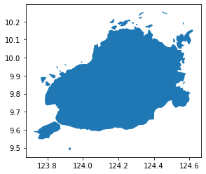
aoi = adm2.loc[adm2.WB_ADM2_NA=='Bohol'].copy()
aoi.plot()
<AxesSubplot:>
3.2. Health Facilities#
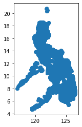
doh = gpd.read_file(os.path.join(input_dir, "doh_healthfacilities_april2020.shp"))
doh.plot()
<AxesSubplot:>
doh = doh.loc[doh.province=='BOHOL'].copy()
doh.head()
| id | facilityco | healthfaci | typeofheal | barangay | municipali | province | region | status | address | style | geometry | |
|---|---|---|---|---|---|---|---|---|---|---|---|---|
| 14672 | 17134.0 | DOH000000000002989 | L.g. Cutamora Community Clinic | Hospital | Fatima | UBAY | BOHOL | REGION VII (CENTRAL VISAYAS) | Functional | Purok 4 | Hospital | POINT (124.47544 10.05558) |
| 15381 | 17135.0 | DOH000000000005353 | Don Emilio Del Valle Memorial Hospital | Hospital | Bood | UBAY | BOHOL | REGION VII (CENTRAL VISAYAS) | Functional | None | Hospital | POINT (124.47465 10.04462) |
| 15601 | 19009.0 | DOH000000000001864 | Clarin Community Hospital | Hospital | Poblacion | CLARIN | BOHOL | REGION VII (CENTRAL VISAYAS) | Functional | Poblacion | Hospital | POINT (124.02349 9.96308) |
| 17029 | 17124.0 | DOH000000000006827 | Ubay Rural Health Unit 1 | Rural Health Unit | Poblacion | UBAY | BOHOL | REGION VII (CENTRAL VISAYAS) | Functional | None | Rural Health Unit | POINT (124.47443 10.05478) |
| 17030 | 17125.0 | DOH000000000024681 | Camambugan Barangay Health Station | Barangay Health Station | Camambugan | UBAY | BOHOL | REGION VII (CENTRAL VISAYAS) | Functional | Purok 4 | Barangay Health Station | POINT (124.43530 10.05757) |
Looking at the NHFR Excel tables received, it looks like there are three separate sheets per region (CV, Cebu, and CAR). Load CV (Central Visaya) and try to match location data from DOH.
registry = pd.read_excel(os.path.join(input_dir, "NHFR_CENTRAL VISAYAS.xlsx"), "CV_7")
registry.columns
Index(['Health Facility Code', 'Health Facility Code Short', 'Facility Name',
       'Old Health Facility Names', 'Old Health Facility Name 2',
       'Old Health Facility Name 3', 'Health Facility Type',
       'Ownership Major Classification',
       'Ownership Sub-Classification for Government facilities',
       'Ownership Sub-Classification for private facilities',
       'Street Name and #           ', 'Building name and #', 'Region Name',
       'Region PSGC', 'Province Name', 'Province PSGC',
       'City/Municipality Name', 'City/Municipality PSGC', 'Barangay Name',
       'Barangay PSGC', 'Zip Code', 'Landline Number', 'Landline Number 2',
       'Fax Number', 'Email Address', 'Alternate Email Address',
       'Official Website', 'Facility Head: Last Name',
       'Facility Head: First Name', 'Facility Head: Middle Name',
       'Facility Head: Position', 'Hospital Licensing Status',
       'Service Capability', 'Bed Capacity'],
      dtype='object')
registry["Province Name"].value_counts()
CEBU               1299
BOHOL               822
NEGROS ORIENTAL     552
SIQUIJOR             67
Name: Province Name, dtype: int64
registry = registry.loc[registry["Province Name"]=="BOHOL"].copy()
registry["Health Facility Type"].value_counts()
Barangay Health Station        687
Rural Health Unit               51
Birthing Home                   51
Hospital                        16
Infirmary                        9
General Clinic Laboratory        5
COVID-19 Testing Laboratory      2
Municipal Health Office          1
Name: Health Facility Type, dtype: int64
len(registry), len(doh)
(822, 546)
registry = registry.merge(doh, left_on='Health Facility Code', right_on='facilityco', how='left')
registry.geometry.isna().value_counts()
False    458
True     376
Name: geometry, dtype: int64
registry = gpd.GeoDataFrame(registry, geometry='geometry', crs=doh.crs)
registry.plot()
<AxesSubplot:>
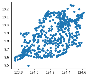
Strategies to match location for missing facilities: look for zip codes, barangay (adm4 file), maybe geocode (not very confident on this last option)
For now work with those that have location
registry = registry.loc[~registry.geometry.isna()].copy()
registry.reset_index(drop=True, inplace=True)
Something important to ask is whether we should be working with health stations. There are hundreds more, so it might be more insightful to consider access to hospitals and primary care centers.
registry_filter = registry.loc[registry["Health Facility Type"]!="Barangay Health Station"].copy()
registry_filter.head(2)
| Health Facility Code | Health Facility Code Short | Facility Name | Old Health Facility Names | Old Health Facility Name 2 | Old Health Facility Name 3 | Health Facility Type | Ownership Major Classification | Ownership Sub-Classification for Government facilities | Ownership Sub-Classification for private facilities | ... | healthfaci | typeofheal | barangay | municipali | province | region | status | address | style | geometry | |
|---|---|---|---|---|---|---|---|---|---|---|---|---|---|---|---|---|---|---|---|---|---|
| 0 | DOH000000000000015 | 15 | CALAPE MAIN HEALTH TB DOTS AND BIRTHING CENTER | CALAPE RURAL HEALTH UNIT | Rural Health Unit | Government | Local Government Unit | ... | Calape Main Health Tb Dots And Birthing Center | Rural Health Unit | Desamparados (pob.) | CALAPE | BOHOL | REGION VII (CENTRAL VISAYAS) | Functional | None | Rural Health Unit | POINT (123.87170 9.89084) | |||
| 1 | DOH000000000000016 | 16 | DAGOHOY RURAL HEALTH UNIT | Rural Health Unit | Government | Local Government Unit | ... | Dagohoy Rural Health Unit | Rural Health Unit | Poblacion | DAGOHOY | BOHOL | REGION VII (CENTRAL VISAYAS) | Functional | None | Rural Health Unit | POINT (124.27175 9.89131) |
2 rows × 46 columns
3.3. Friction Surface#
wp_1km = os.path.join(input_dir, "phl_ppp_2020_1km_Aggregated_UNadj.tif")
inP = rio.open(wp_1km)
# Clip the pop raster to AOI
out_pop = os.path.join(out_folder, "pop_bohol.tif")
# rMisc.clipRaster(inP, aoi, out_pop, bbox=False, buff=0.1)
pop_surf = rio.open(out_pop)
# standardize so that they have the same number of pixels and dimensions
out_pop_surface_std = os.path.join(out_folder, "pop_bohol_STD.tif")
# rMisc.standardizeInputRasters(pop_surf, travel_surf, out_pop_surface_std, resampling_type="nearest")
# create a data frame of all points
pop_surf = rio.open(out_pop_surface_std)
pop = pop_surf.read(1, masked=True)
indices = list(np.ndindex(pop.shape))
xys = [Point(pop_surf.xy(ind[0], ind[1])) for ind in indices]
res_df = pd.DataFrame({
    'spatial_index': indices,
    'xy': xys,
    'pop': pop.flatten()
})
res_df['pointid'] = res_df.index
# drop non-populated points
res_df = res_df.loc[res_df['pop']>0].copy()
res_df = res_df.loc[~(res_df['pop'].isna())].copy()
# res_df.loc[:,'xy'] = res_df['xy'].apply(Point)
res_gdf = gpd.GeoDataFrame(res_df, geometry='xy', crs='EPSG:4326')
len(res_df), len(registry_filter)
(5194, 71)
3.4. Catchment Area#
For every health facility, calculate travel time between origin point and health facility. Then for each point, keep the id of the health facility with the minimum travel time (closest idx) using Mapbox!
res_gdf.head()
| spatial_index | xy | pop | pointid | hrs_to_hosp_or_clinic | mins_to_hosp_or_clinic | dist_to_hosp_or_clinic | closest_hosp_or_clinic_id | closest_hosp_or_clinic_name | closest_hosp_or_clinic_geom_lon_x | closest_hosp_or_clinic_geom_lat_y | closest_hosp_or_clinic_geodetic_dist | mb_snapped_dest_name | mb_snapped_dest_dist | mb_snapped_dest_lon_x | mb_snapped_dest_lat_y | mb_snapped_src_name | mb_snapped_src_dist | mb_snapped_src_lon_x | mb_snapped_src_lat_y | |
|---|---|---|---|---|---|---|---|---|---|---|---|---|---|---|---|---|---|---|---|---|
| 1583 | (11, 120) | POINT (124.62083 10.26250) | 233.189651 | 1583 | -1 | -1 | -1 | -1 | -1 | -1 | -1 | -1 | -1 | -1 | -1 | -1 | -1 | -1 | -1 | -1 |
| 1676 | (12, 80) | POINT (124.28750 10.25417) | 94.150398 | 1676 | -1 | -1 | -1 | -1 | -1 | -1 | -1 | -1 | -1 | -1 | -1 | -1 | -1 | -1 | -1 | -1 |
| 1677 | (12, 81) | POINT (124.29583 10.25417) | 362.527374 | 1677 | -1 | -1 | -1 | -1 | -1 | -1 | -1 | -1 | -1 | -1 | -1 | -1 | -1 | -1 | -1 | -1 |
| 1682 | (12, 86) | POINT (124.33750 10.25417) | 24.213766 | 1682 | -1 | -1 | -1 | -1 | -1 | -1 | -1 | -1 | -1 | -1 | -1 | -1 | -1 | -1 | -1 | -1 |
| 1695 | (12, 99) | POINT (124.44583 10.25417) | 176.003372 | 1695 | -1 | -1 | -1 | -1 | -1 | -1 | -1 | -1 | -1 | -1 | -1 | -1 | -1 | -1 | -1 | -1 |
res_gdf.loc[:, "geometry"] = res_gdf.xy
registry_filter.loc[:, "idx"] = registry_filter.index
registry_filter.loc[:, "name"] = registry_filter.loc[:, "Health Facility Code"]
# visual= plot_df_single(res_gdf, 'xy', color = 'blue', alpha = 0.8, hover_cols=['pop'])
origins_driving = get_travel_times_mapbox(
    origins = res_gdf,
    destinations = registry_filter,
    mode = 'driving',
    d_name = False,
    dest_id_col = "idx",
    n_keep = 2,
    num_retries = 2,
    starting_token_index = 0,
    use_pickle=False,
    do_pickle_result=False
)
for idx, dest in registry.iterrows():
    dest_gdf = gpd.GeoDataFrame([dest], geometry='geometry', crs='EPSG:4326')
    res = ma.calculate_travel_time(travel_surf, mcp, dest_gdf)[0]
    res_df.loc[:,idx] = res.flatten()
# drop non-populated points
res_df = res_df.loc[res_df['pop']>0].copy()
res_df = res_df.loc[~(res_df['pop'].isna())].copy()
# res_df.loc[:, registry.index] = res_df.loc[:, registry.index].apply(lambda x: x/60) # convert to hours
res_df.head()
| spatial_index | xy | pop | pointid | 0 | 1 | 2 | 3 | 4 | 5 | ... | 448 | 449 | 450 | 451 | 452 | 453 | 454 | 455 | 456 | 457 | |
|---|---|---|---|---|---|---|---|---|---|---|---|---|---|---|---|---|---|---|---|---|---|
| 1583 | (11, 120) | POINT (124.62083333333334 10.262500000000001) | 233.189651 | 1583 | 174.827661 | 112.596690 | 132.981467 | 126.174397 | 125.830508 | 89.194147 | ... | 83.001395 | 80.219273 | 125.275623 | 124.507856 | 58.504034 | 127.471059 | 114.321564 | 97.282982 | 100.968181 | 182.230204 |
| 1676 | (12, 80) | POINT (124.28750000000001 10.254166666666668) | 94.150398 | 1676 | 104.289856 | 70.685185 | 91.069961 | 109.733454 | 109.389565 | 44.628835 | ... | 86.853345 | 57.760563 | 54.737817 | 53.970050 | 58.188452 | 97.456000 | 85.513612 | 55.371476 | 35.676160 | 140.318698 |
| 1677 | (12, 81) | POINT (124.29583333333333 10.254166666666668) | 362.527374 | 1677 | 103.594973 | 69.990302 | 90.375078 | 109.038572 | 108.694682 | 43.933953 | ... | 86.158463 | 57.065681 | 54.042935 | 53.275168 | 56.653935 | 96.761117 | 84.818729 | 54.676594 | 34.981278 | 139.623816 |
| 1682 | (12, 86) | POINT (124.3375 10.254166666666668) | 24.213766 | 1682 | 113.083750 | 73.920799 | 94.305575 | 112.850695 | 112.506806 | 47.864450 | ... | 87.198279 | 58.984406 | 63.531712 | 62.763945 | 40.853934 | 100.691614 | 88.749226 | 58.607090 | 36.106657 | 143.554312 |
| 1695 | (12, 99) | POINT (124.44583333333334 10.254166666666668) | 176.003372 | 1695 | 123.820979 | 79.887000 | 100.271776 | 115.157095 | 114.813206 | 52.366185 | ... | 89.038979 | 61.290806 | 74.268941 | 73.501174 | 2.474874 | 106.657815 | 94.715427 | 64.573291 | 45.570285 | 149.520514 |
5 rows × 462 columns
res_df.loc[:, "closest_idx"] = res_df[registry.index].idxmin(axis=1) # id of health facility that yields the minimum travel time
res_df.loc[:, "closest_idx_filter"] = res_df[registry_filter.index].idxmin(axis=1) # same but without health stations
res_df.loc[:,'xy'] = res_df['xy'].apply(Point)
res_gdf = gpd.GeoDataFrame(res_df, geometry='xy', crs='EPSG:4326')
#libraries for plotting maps
import matplotlib.pyplot as plt
import matplotlib.colors as colors
from rasterio.plot import plotting_extent
import contextily as ctx
import random
3.4.1. Save some maps#
Issue here is that the colors are being repeated and grouped
graphs_dir = os.path.join(repo_dir, 'output')
if not os.path.exists(graphs_dir):
    os.mkdir(graphs_dir)
figsize = (12,12)
fig, ax = plt.subplots(1, 1,  figsize = figsize)
ax.set_title("Closest health facility for each grid point", fontsize=14)
res_gdf.plot('closest_idx', ax = ax, categorical=True, legend=False)
plt.axis('off')
ctx.add_basemap(ax, source=ctx.providers.Stamen.Terrain, crs='EPSG:4326', zorder=-10)
registry.plot(ax=ax, facecolor='black', edgecolor='white', markersize=30, alpha=1)
plt.savefig(os.path.join(graphs_dir, "Bohol_Catchment_AllHealth.png"), dpi=300, bbox_inches='tight', facecolor='white')
<AxesSubplot:title={'center':'Closest health facility for each grid point'}>
# spec = plt.cm.get_cmap('tab20c')
number_of_colors = len(res_gdf.closest_idx_filter.unique())

color = ["#"+''.join([random.choice('0123456789ABCDEF') for j in range(6)])
             for i in range(number_of_colors)]

custom = colors.ListedColormap(color)
figsize = (12,12)
fig, ax = plt.subplots(1, 1, figsize = figsize)
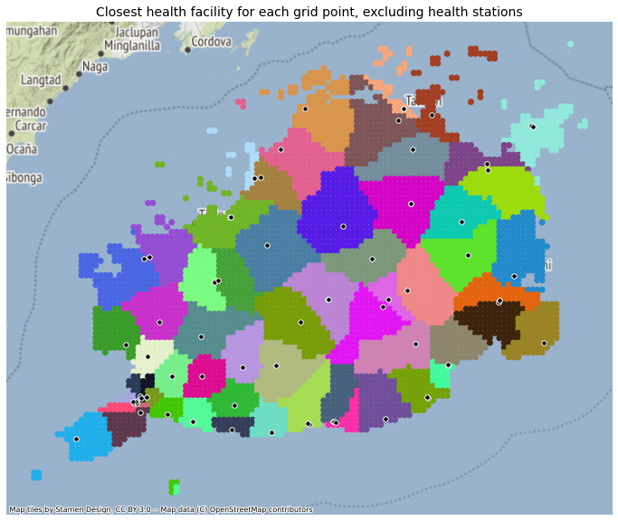
ax.set_title("Closest health facility for each grid point, excluding health stations", fontsize=14)
res_gdf.plot('closest_idx_filter', ax = ax, categorical=True, legend=False, cmap=custom)
plt.axis('off')
ctx.add_basemap(ax, source=ctx.providers.Stamen.Terrain, crs='EPSG:4326', zorder=-10)
registry_filter.plot(ax=ax, facecolor='black', edgecolor='white', markersize=30, alpha=1)
plt.savefig(os.path.join(graphs_dir, "Bohol_Catchment_NoStations.png"), dpi=300, bbox_inches='tight', facecolor='white')
<AxesSubplot:title={'center':'Closest health facility for each grid point, excluding health stations'}>
3.4.2. Calculate travel time to nearest health facility (excluding stations)#
pop_surf = rio.open(out_pop_surface_std)
pop = pop_surf.read(1, masked=True)
indices = list(np.ndindex(pop.shape))
xys = [Point(pop_surf.xy(ind[0], ind[1])) for ind in indices]
res_df = pd.DataFrame({
    'spatial_index': indices,
    'xy': xys,
    'pop': pop.flatten()
})
res_df['pointid'] = res_df.index
# same analysis but we feed all destinations at once, this returns the travel time to closest
res_min = ma.calculate_travel_time(travel_surf, mcp, registry_filter)[0]
res_df.loc[:, f"tt_health"] = res_min.flatten()
res_df = res_df.loc[res_df['pop']>0].copy()
res_df = res_df.loc[~(res_df['pop'].isna())].copy()
res_df.head()
| spatial_index | xy | pop | pointid | tt_health | |
|---|---|---|---|---|---|
| 1583 | (11, 120) | POINT (124.6208333333333 10.2625) | 233.189651 | 1583 | 54.864499 |
| 1676 | (12, 80) | POINT (124.2875 10.25416666666667) | 94.150398 | 1676 | 35.676160 |
| 1677 | (12, 81) | POINT (124.2958333333333 10.25416666666667) | 362.527374 | 1677 | 34.981278 |
| 1682 | (12, 86) | POINT (124.3375 10.25416666666667) | 24.213766 | 1682 | 36.106657 |
| 1695 | (12, 99) | POINT (124.4458333333333 10.25416666666667) | 176.003372 | 1695 | 39.898555 |
res_df.tt_health.describe()
count    5194.000000
mean       11.641249
std        11.376083
min         0.000000
25%         4.767767
50%         8.293451
75%        13.958109
max       120.100080
Name: tt_health, dtype: float64
These values seem really low! (minutes)
Maybe becuase it’s an island? We need to do some checks…
res_df.loc[:,'xy'] = res_df['xy'].apply(Point)
res_gdf_tt = gpd.GeoDataFrame(res_df, geometry='xy', crs='EPSG:4326')
figsize = (12,12)
fig, ax = plt.subplots(1, 1, figsize = figsize)
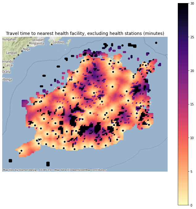
ax.set_title("Travel time to nearest health facility, excluding health stations (minutes)", fontsize=14)
res_gdf_tt.plot('tt_health', ax = ax, categorical=False, legend=True, vmin=0, vmax=30, cmap='magma_r')
plt.axis('off')
ctx.add_basemap(ax, source=ctx.providers.Stamen.Terrain, crs='EPSG:4326', zorder=-10)
registry_filter.plot(ax=ax, facecolor='black', edgecolor='white', markersize=50, alpha=1)
plt.savefig(os.path.join(graphs_dir, "Bohol_TravelTime_NoStations.png"), dpi=300, bbox_inches='tight', facecolor='white')
# res_min[res_min>99999999] = np.nan
# res_min = res_min/60
# from mpl_toolkits.axes_grid1 import make_axes_locatable
# figsize = (12,12)
# fig, ax = plt.subplots(1, 1,  figsize = figsize)
# ax.set_title("Travel time to nearest health facility", fontsize=14)

# plt.axis('off')
# ext = plotting_extent(pop_surf)

# im = ax.imshow(res_min, vmin=0, vmax=1, cmap='magma_r', extent=ext)
# # im = ax.imshow(res_min, norm=colors.PowerNorm(gamma=0.05), cmap='YlOrRd', extent=ext)
# # im = ax.imshow(res_min, cmap=newcmp, extent=ext)

# # ctx.add_basemap(ax, source=ctx.providers.Esri.WorldShadedRelief, crs='EPSG:4326', zorder=-10)
# ctx.add_basemap(ax, source=ctx.providers.Stamen.Terrain, crs='EPSG:4326', zorder=-10)

# registry_filter.plot(ax=ax, facecolor='black', edgecolor='white', markersize=50, alpha=1)
# aoi.plot(ax=ax, facecolor='none', edgecolor='black')

# divider = make_axes_locatable(ax)
# cax = divider.append_axes('right', size="4%", pad=0.1)
# cb = fig.colorbar(im, cax=cax, orientation='vertical')

# plt.savefig(os.path.join(graphs_dir, "Bohol_TravelTime_NoStations.png"), dpi=300, bbox_inches='tight', facecolor='white')
# # fig = ax.get_figure()
# # fig.savefig(
# #     os.path.join(out_folder, "MNG_AirportTravelTime.png"),
# #     facecolor='white', edgecolor='none'
# # )
Save some output data to check values
registry.loc[:, "idx"] = registry.index
registry.to_file(os.path.join(out_folder, "registry.shp"))
raster_path = out_pop_surface_std
res_gdf.loc[:, "geometry"] = res_gdf.loc[:, "xy"]
res_gdf.loc[:, "closest_idx"] = res_gdf.loc[:, "closest_idx"].astype('int32')
aggregator.rasterize_gdf(res_gdf, 'closest_idx', raster_path, os.path.join(out_folder, "closest_idx_.tif"), nodata=-1)